Welcome

This notebook contains my personal notes for CS7646: Machine Learning for Trading, offered at the Georgia Institute of Technology. A summary of the course follows:

This course introduces students to the real world challenges of implementing machine learning based trading strategies including the algorithmic steps from information gathering to market orders. The focus is on how to apply probabilistic machine learning approaches to trading decisions. We consider statistical approaches like linear regression, Q-Learning, KNN, and regression trees and how to apply them to actual stock trading situations.

Course links:

• https://omscs.gatech.edu/cs-7646-machine-learning-trading

Part 1

The following section contains my notes for Part 1 of the course "CS 7646: Machine Learning for Trading". This section of the course covers the manipulation of financial data using Python.

1-1: Reading and plotting stock data

This lesson contains a basic introduction to the manipulation of data using Python. Most of the data provided in this course comes in the format of .csv files.

What does real stock data look like?

Usually, each .csv file containing stock data is named after its respective stock symbol. We can expect the following headers in the stock's .csv file:

• Date
• Open
• High
• Low
• Close
• Volume
• Adjusted Close (Adj Close)

Each .csv file is sorted from newest to oldest record, based upon the Date field.

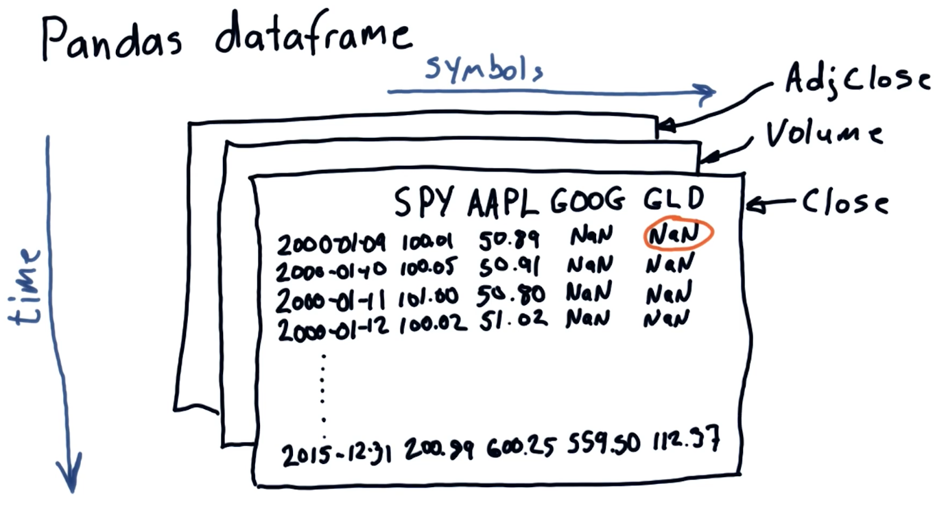
The pandas dataframe

pandas is a Python library used to manipulate large sets of data. When pandas ingests .csv, it stores the rows and columns in a certain format, or dataframe, that allows us to easily access different sets of data programmatically. Below is an example drawing from the class of the Pandas dataframe, each plane of the dataframe is separated by the headers we listed above: Close, Volume, Adj Close, etc.

Quizzes

Which fields would you expect to see in a .csv file of stock data?

• Number of employees
• Date / time
• Company name
• Price of the stock
• Company's hometown

1-2: Working with multiple stocks

This lesson covers more in-depth manipulation of stock data in .csv files with pandas. In this lesson, we create empty dataframes with pandas and selectively include data from a number of .csv files of different stock symbols. This lesson provides examples of selecting stock information based upon date ranges from various stock symbols, and provides guidance on how to avoid ingesting invalid (NaN values) into the dataframe. An example provided by the lesson can be found here.

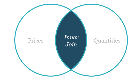
Inner join vs outer join

An inner join of a table provides the common items between the two tables being joined. An example Venn-diagram of the operation is provided below:

An outer join of a table provides the common items between two tables, as well, however it also provides the left or right quantities of the two tables being joined. An example Venn-diagram of a left outer join and a right outer join are provided below:

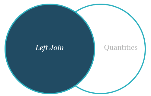
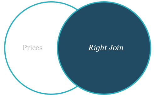
The default method of join for a pandas dataframe is the left outer join.

Normalizing price data

The preferred method to normalize data within a pandas dataframe is to conduct the following operation in Python:

my_dataframe = my_dataframe / mydataframe.ix[0, :]

Quizzes

How many days were U.S. stocks traded at NYSE in 2014?

• 365
• 260
• 252

1-3: The power of NumPy

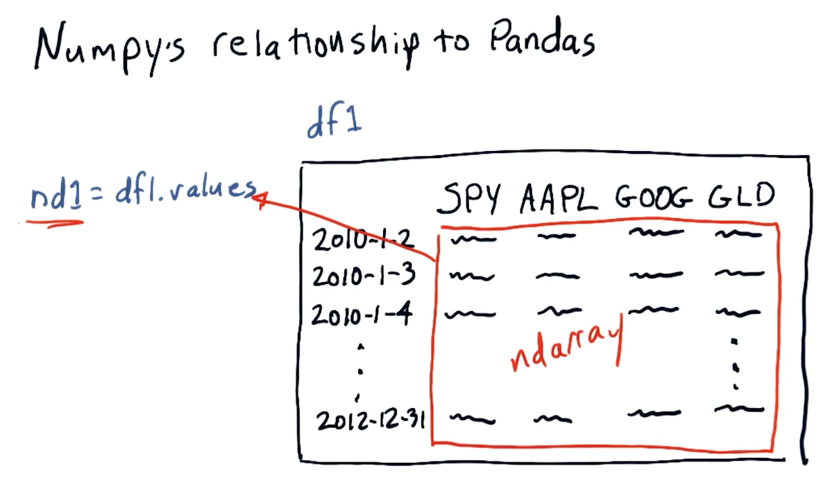
NumPy's relationship to Pandas

pandas is essentially a wrapper for numpy ndarray objects. Below is a screenshot from the lectures providing a conceptual overview of the objects' relationships:

1-4: Statistical analysis of time series

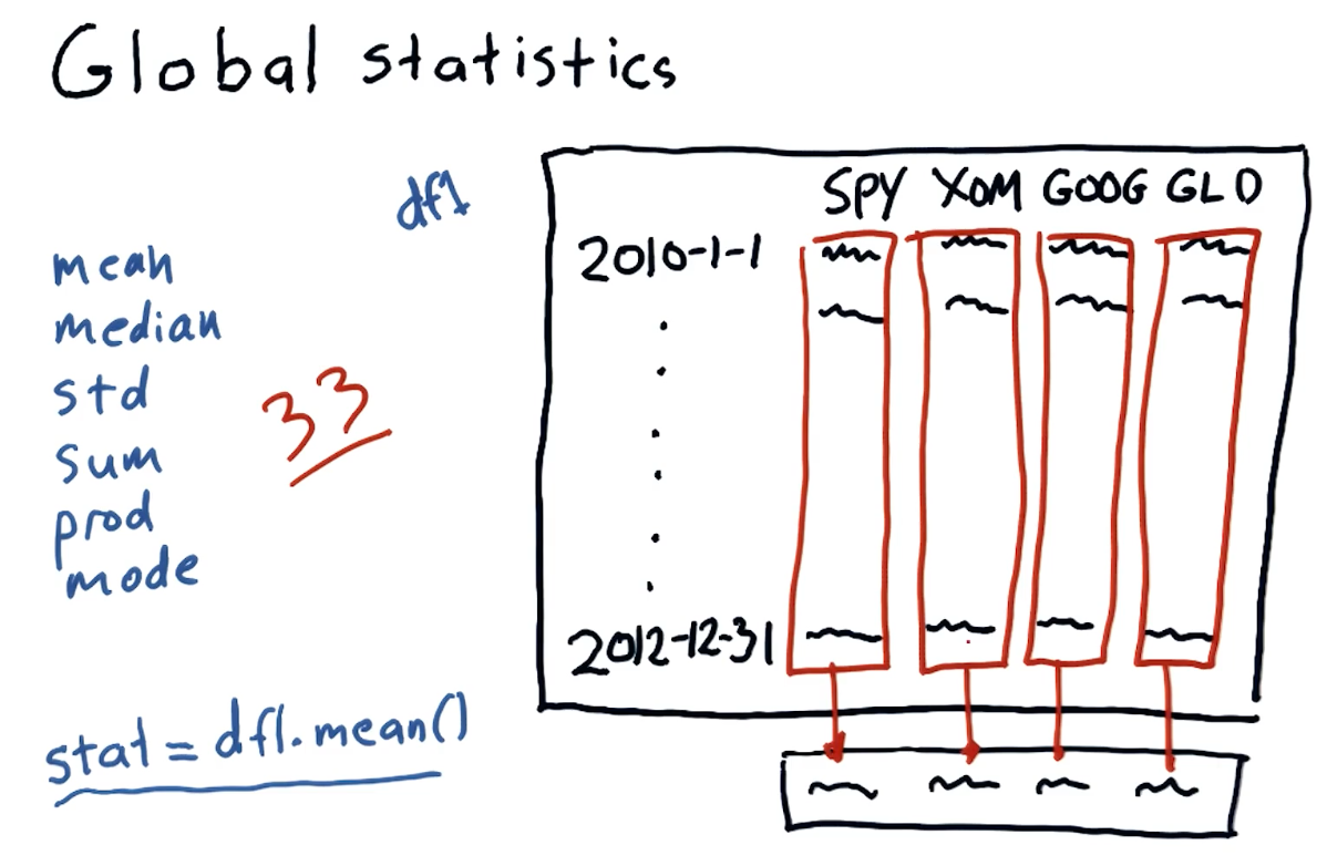
Global statistics

We can easily compute global statistics like mean, median, standard deviation, and more using pandas dataframes. A high-level interpretation provided in the course lecture is provided below:

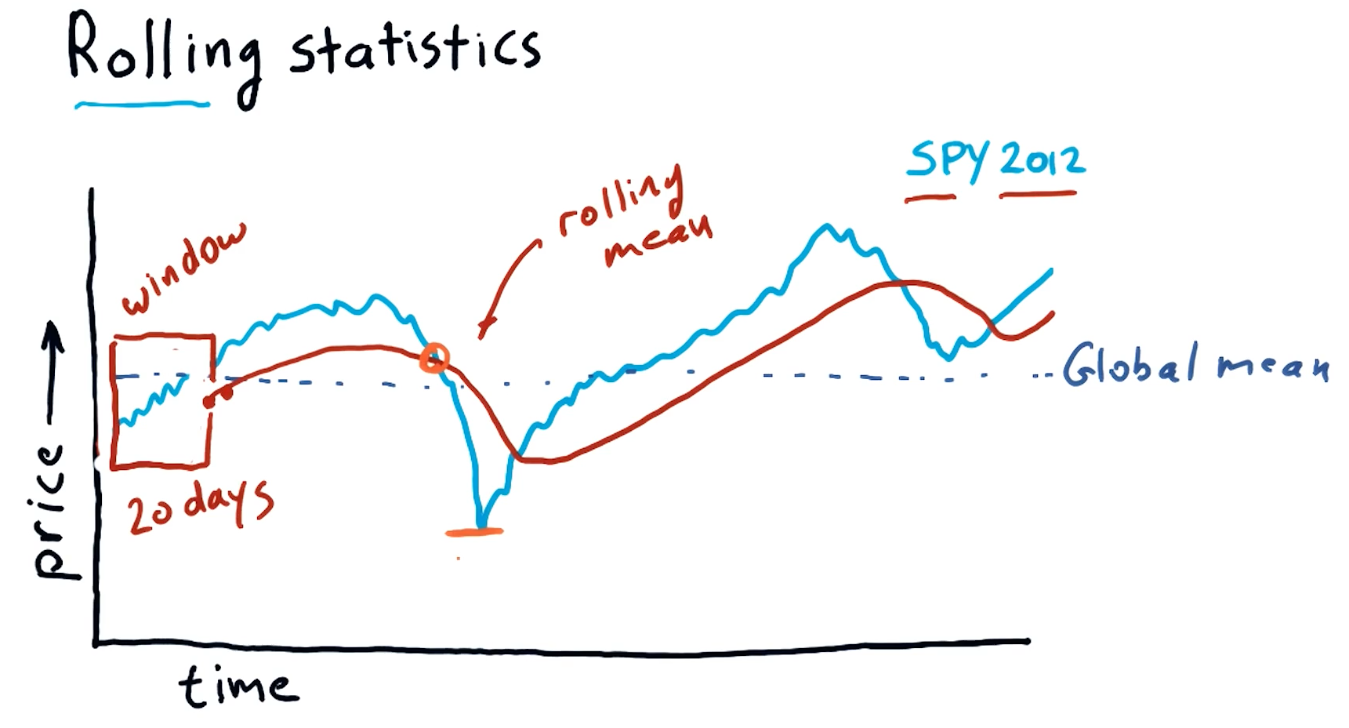
Rolling statistics

Rolling statistics are statistics observed during a time-slice of the global data. These rolling statistics allow us to derive trends from the global data. A high-level interpretation provided in the course lecture is provided below:

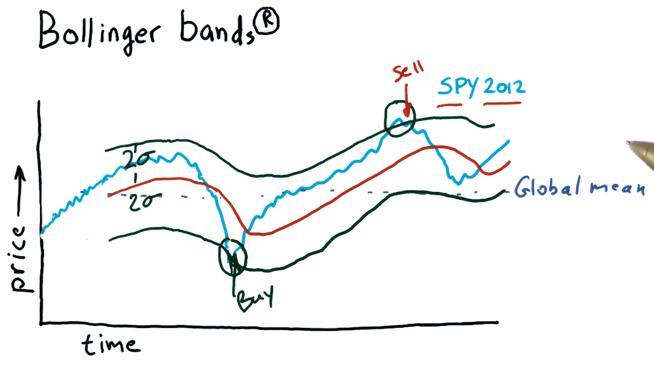
Bollinger bands

Bollinger bands are a trading concept where we maintain a rolling mean and define two bands that are separated two standard deviations from the rolling mean in both directions. Once a stock's value crosses below the lower threshold and then crosses above it, we can consider this a buy signal. Similarly, we can detect a sell signal when a stock crosses above the higher threshold and begins to dip below it. A high-level interpretation provided in the course lecture is provided below:

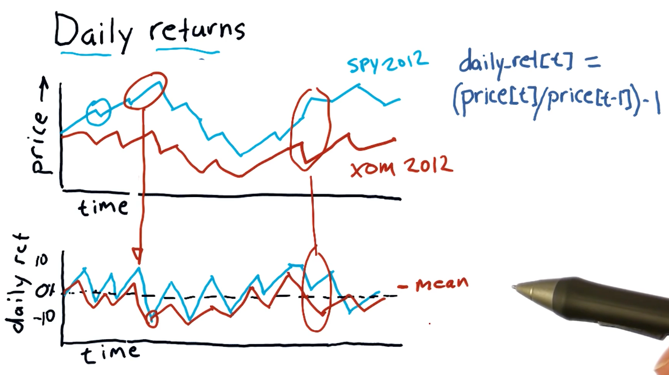
Daily returns

Daily returns can be easily calculated using the following equation:

• daily_ret(t) = (price[t] / price[t-1]) - 1

Where t == date.

A high-level representation of daily returns from the course lecture is provided below:

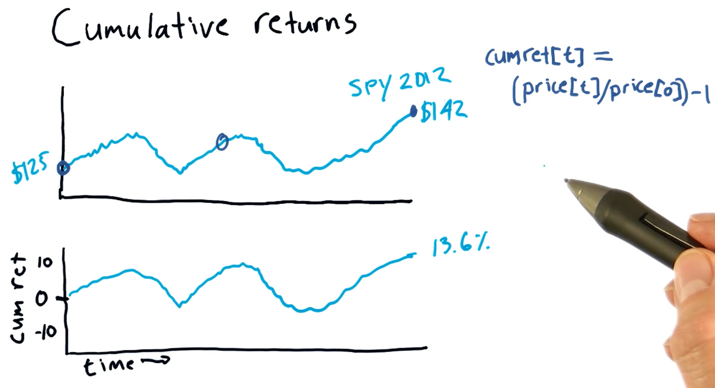
Cumulative returns

Cumulative returns can be easily calculated using the following equation:

• cumulative_ret(t) = (price[t] / price[0]) - 1

A high-level representation of cumulative returns from the course lecture is provided below:

Quizzes

Which statistic is best to use to determine buy / sell signals?

• rolling sum
• global mean
• global max
• rolling standard deviation

1-5: Incomplete data

While we might think financial data is well documented, sometimes financial data that we want to inspect can be missing from public archives. This lesson covers how we can mitigate the consequences of missing financial data.

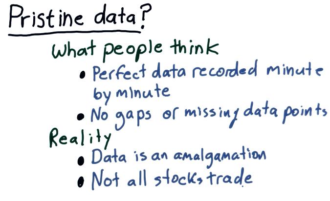
Pristine data

Below is a screenshot from the lecture listing some of the issues with incomplete financial data:

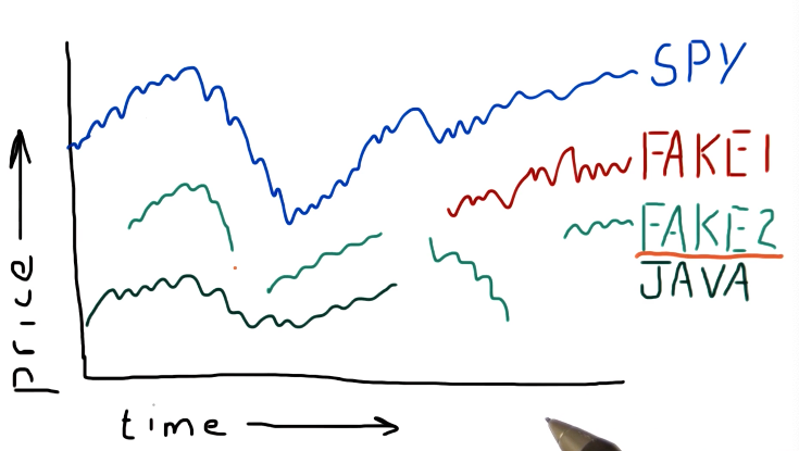
Why data goes missing

From the lecture, some examples are given as to why stocks disappear or appear in the data / timeline. Some stocks get acquired by different companies, so companies completely go under and are no longer traded, and some stocks appear in the middle of the timeline because they are newer. A high-level representation from the lecture is provided below:

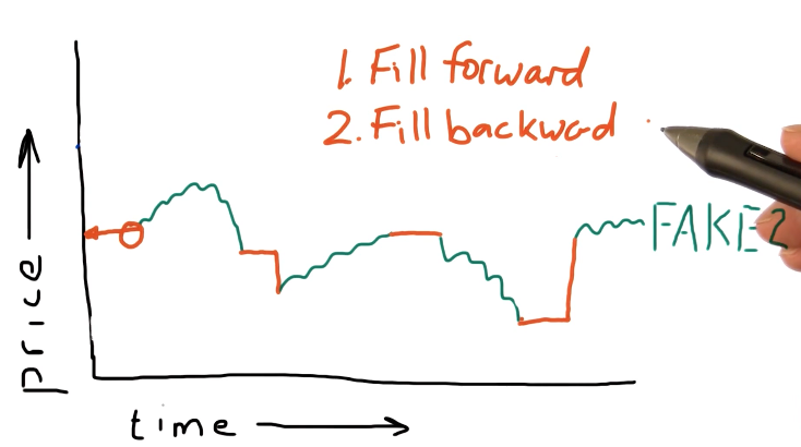
What can we do?

Pandas provides us with the ability to fill forward and fill backwards missing data between two points in time with the last known-good data point. It's best practice to fill forward first and then fill backwards. A high-level representation of this concept is from the lecture is provided below:

Pandas fillna()

Pandas provides us with a powerful function called fillna() that can be used with dataframes to fill forward or fill backwards missing values.

1-6: Histograms and scatter plots

This lesson covers how to utilize histograms and scatter plots to analyze and compare daily returns of multiple stocks. This is a more useful technique than analyzing a stock by itself.

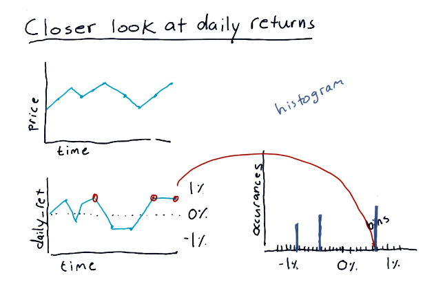
Daily returns

This section discusses what a histogram looks like and what information it captures. A high-level representation of a histogram in comparison with a stock price and daily returns graph can be found below:

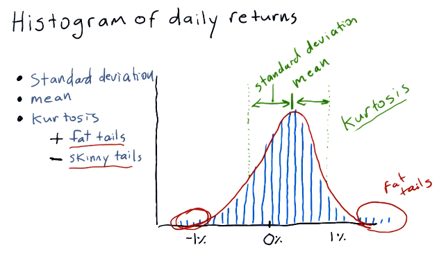
Histogram of daily returns

In the below example, the lecture discusses the normal shape of a histogram which, like most things, is a bell curve. The lecture discusses the concept of kurtosis, describing fat tails and skinny tails - a measurement of the distribution of the histogram.

Fat tails mean that there are a large number of occurrences happening on the outer edges of the distribution, meanwhile skinny tails indicate the opposite. Below is a high-level representation of these concepts:

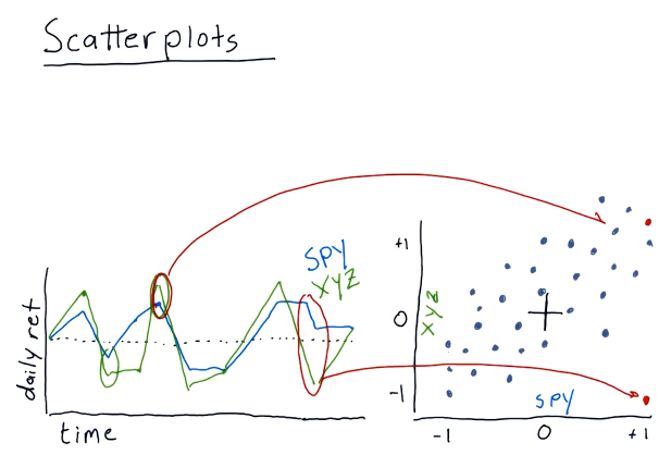
Scatterplots

This section discusses how scatterplots are generated to compare two stocks. As we can see, general trends begin to form when a scatterplot is generated for two stocks, allowing us to infer about the behavior or performance for a particular stock. Below is a high-level representation provided by the lecture:

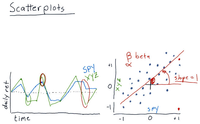
Scatterplot slopes

In this section of the lecture, alpha and beta are described for a given scatterplot. alpha and beta are both functions of the slopes of the possible lines that can be drawn for a given scatterplot. Beta describes how reactive a particular stock is to the market. If the market goes up by %1, this stock would also achieve %1 - if the beta was equal to one. If the beta was equal to two, the stock would achieve %2 while the market achieved %1.

In a similar vein, we have alpha - the intersection between the line we've drawn using the scatterplot and the vertical axis. alpha describes how a stock performs on average better than market making stocks like the S&P500.

A high-level representation of these concepts is provided below:

Correlation

Correlation is a measurement of how close the dots on a scatterplot are to the line we've drawn through the scatterplot.

1-7: Sharpe ratio and other portfolio statistics

In this lesson we cover portfolio statistics used in the real world and how to calculate and interpret these statistics using Python.

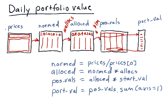
Daily portfolio values

Given a starting investment amount, allocation percentages to respective stocks, and a window in time to conduct calculations, we can calculate the daily value of a portfolio over a given period of time.

Taking the prices dataframe, we can normalize the data and apply a series of transforms to arrive at an array of values describing our portfolio's daily value over a given period of time. Below is a high-level interpretation of how to achieve this outcome given a dataframe:

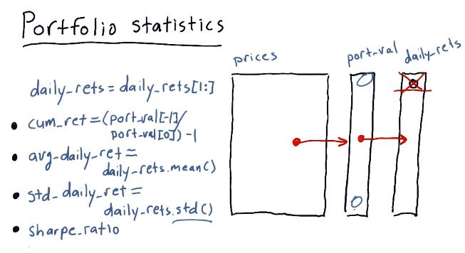
Portfolio statistics

Using our new portfolio value array, we can calculate a series of important statistics, such as:

• cumulative return
• average daily return
• standard daily return
• sharpe ratio

A high-level interpretation from the lecture is provided below. This image also provides the equations to derive the statistics listed above:

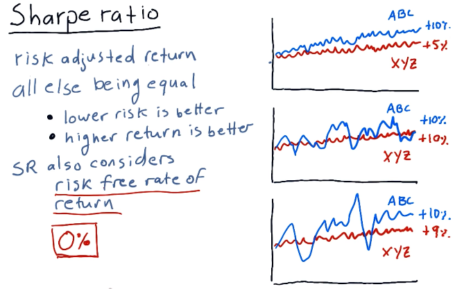
Sharpe ratio

The sharpe ratio of a portfolio is a statistic that adjusts overall return for risk apparent in the portfolio. This is mostly useful when comparing two stocks or portfolio wherein one has a greater return but poses a greater risk - it allows us to make an informed decision about the riskier of the two stocks.

A high-level representation of these concepts from the lectures is provided below:

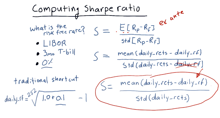
Computing sharpe ratio

To compute the sharpe ratio we need to divide the Expected Value of the portfolio returns minus the risk free rate by the standard deviation of the portfolio returns minus the risk free rate. The slide from the lectures, below, provides possible references for the risk free rate, however, traditionally it's been 0.

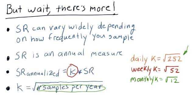
Sharpe ratio frequency

The sharpe ratio can be affected by the frequency in which sampling of the portfolio occurs - it was originally intended to be an annual measure. In order to acquire the annualized version of the sharpe ratio, you multiply the sharpe ratio result by the constant k. This is calculated by taking the square root of the frequency of sampling. The slide from the lecture provides more insight into how the sharpe ratio is affected by frequency:

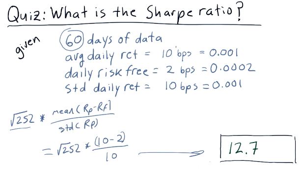
Quizzes

What is the sharpe ratio?

Below is a quiz from the class providing us with a scenario to calculate the sharp ratio with concrete values:

1-8: Optimizers

This lesson covers optimizers, algorithms that can do the following:

• Find the minimum values of functions
• Build parameterized models based on data
• Refine allocations to stocks in portfolios

To use an optimizer, we conduct the following steps:

1. Provide a function to minimize
2. Provide an initial guess of what the minimal outcome is
3. Call the optimizer repeatedly until we reach the minimum

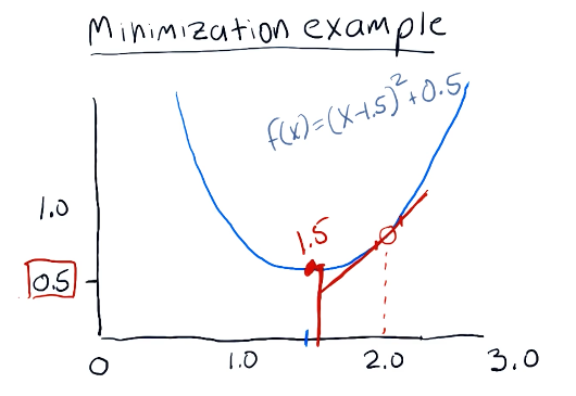
Minimization example

The following example for minimization is provided by the lecture. The minimizer in this example continues to test values for the given equation, tracking the minimum value until it reaches the lowest possible number. This algorithm rejects values that are high than it's most recent minimum, and continues to search for the lowest possible value with greater granularity as it completes iterations of the minimization algorithm.

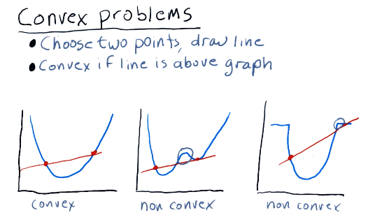
Convex problems

When finding the minima of a given equation, we can run into an issue for complex equations or convex problems. In these problems, the minima can be difficult to find for a traditional minimizing algorithm due to the odd shape of the equation when graphed. It can have local minima, or portions of the line that plateau. Below is a slide from the lecture demonstrating this problem and how a minimization algorithm could solve it:

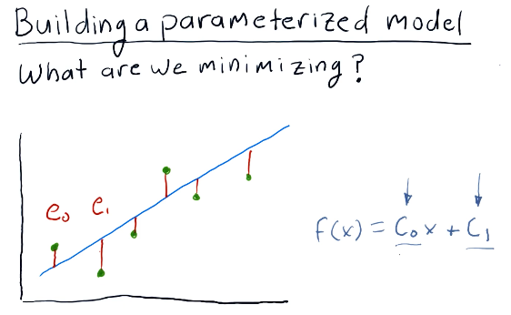
Building a parameterized model

Given a scatterplot like the one shown below from the lecture, a minimizer can determine the coefficients for a given equation by minimizing the distance of a graphed line (from the equation) to the dots on the scatterplot. This distance is known as error. The minimizer will attempt to minimize the amount of error, finding the appropriate coefficients.

1-9: How to optimize a portfolio

What is portfolio optimization?

Given a set of assets and a time period, find an allocation of funds to assets that maximizes performance.

What is performance?

We can choose from a number of statistics such as:

• Cumulative returns
• Volatility or risk
• Risk adjusted returns (Sharpe ratio)

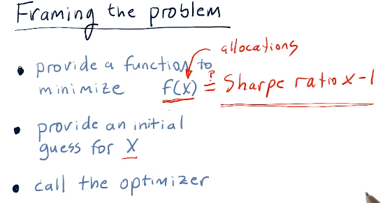
Framing the problem

So how do we go about optimizing a portfolio? We use an optimizer to find the inverse Sharpe ratio for a given set of allocations in a portfolio. A high-level representation provided by the lecture is provided below:

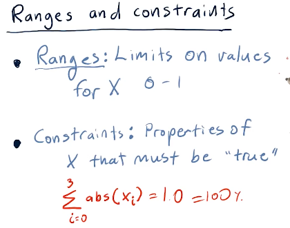
Ranges and constraints

Ranges and constraints on the values of X provided to the optimizer for the function to be minimized can help speed-up the rate at which the optimize can solve the minimization of the function. Ranges in this case should be limited from 0 to 1 as these represent percentages. Constraints in this example specify that the sum(x) should equal 100 - meaning our allocations reach 100% for an effectively optimized portfolio. Below is the slide from the lecture discussing this topic:

Part 2

The following section contains my notes for Part 2 of the course "CS 7646: Machine Learning for Trading". This section of the course covers computational investing.

2-1: So you want to be a hedge fund manager?

This lesson covers the fundamentals of being a portfolio manager.

Types of funds

The following are types of funds:

• ETFs - exchange traded funds
  • Buy and sell like stocks
  • Represent baskets of stocks
  • Transparent
• Mutual funds
  • Buy and sell at the end of the trading day
  • Quarterly disclosure
  • Less transparent
• Hedge funds
  • Buy and sell by agreement
  • No disclosure
  • Not transparent

Incentives: How are they compensated?

• ETFs - Managers of ETFs are compensated according to an expense ratio, related to AUM.
• Mutual funds - Compensated according to an expense ratio, usually much higher than ETFs.
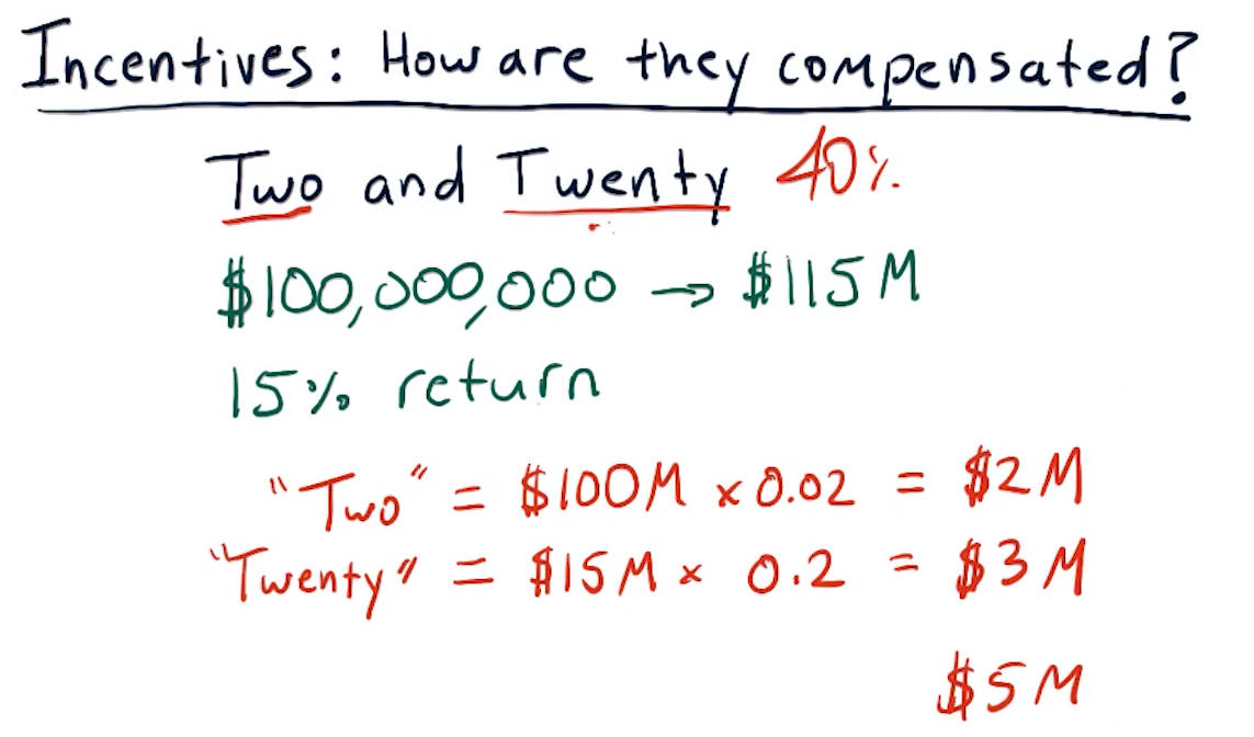
• Hedge funds - Follow an old model called two and twenty.

Two and twenty

Below is a breakdown from the lectures on how the two and twenty compensation model works for hedge fund managers:

How do hedge funds attract investors?

Hedge funds are usually designed to attract and do business with the following entities:

• Individuals - usually particularly wealthy individuals because hedge funds are on average only made up of 100 people
• Institutions - institutions like Harvard or Georgia Tech that want to park assets and watch them accrue in value
• Funds of funds

Why would one of these entities pick a particular hedge fund over another?:

• Track record - potential investors will always review the track record of a particular fund. The fund should have no less than 5 years of maturity.
• Simulation and story - potential investors would like to see the backtesting results of a particular strategy, and a story as to why the hedge fund manager believes their strategy is novel or successful.
• Good portfolio fit - potential investors will be on the lookout to find a portfolio they don't already have. It's like investors will not invest into a hedge fund that already covers a sector of the market they have assets in.

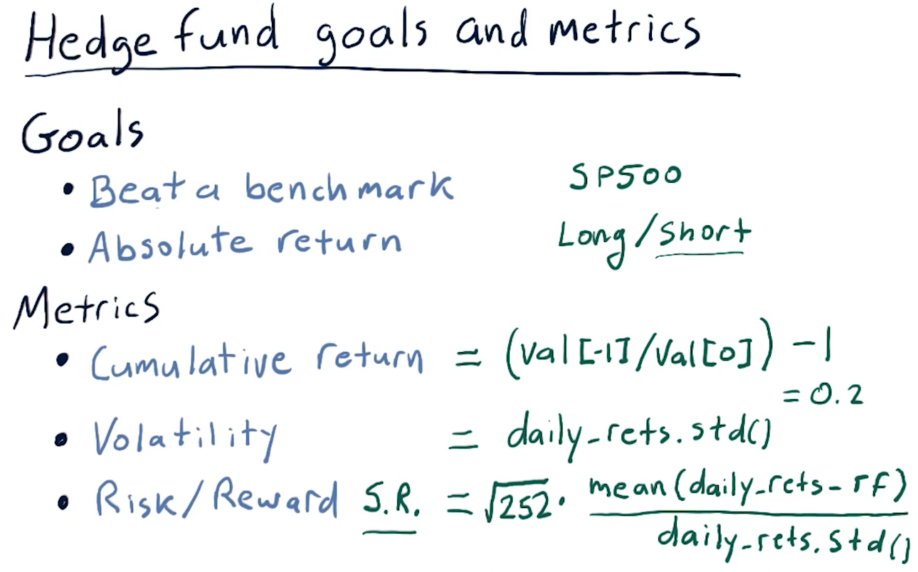
Hedge fund goals and metrics

Hedge funds usually have one of the two following goals:

• Beat a benchmark - following or beating a benchmark like the SP500
  • Riskier because it usually follows the market and its trends.
• Absolute return - playing long and short positions so that, at the end of the year, the fund is positive.
  • Usually doesn't have large returns, but a safe bet to always have positive returns.

We calculate the metrics like we've done in other lessons. You can find the lecture slide for this section of the lesson, below:

The computing inside a hedge fund

The lecture provides us with a high-level overview of computing within a hedge fund, this can be found below. One thing to note with this image is that, if the hedge fund wanted to enter a particular position, e.g. purchase 1 mil worth of AAPL stock, the trading algorithm isn't going to create a BUY signal to conduct this immediately. The trading algorithm leverages feedback from the market and executes orders incrementally to avoid influencing the market too much while allowing the fund to enter a particular position.

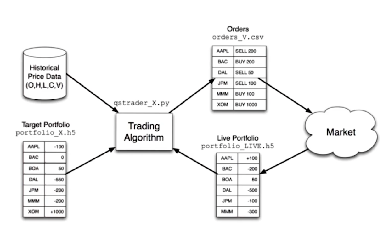
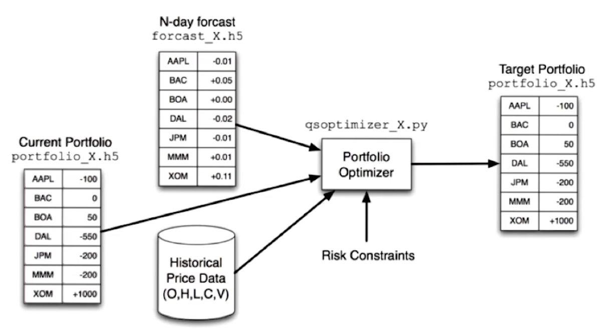
Up next, the lecture provides us with how target portfolios are calculated. This is typically done using an optimizer like we've seen in previous lessons. The optimizer leverages inputs from a forecaster, the current portfolio, historical price data, and some risk constraints provided by the hedge fund manager. A high-level overview of this concept is provided below:

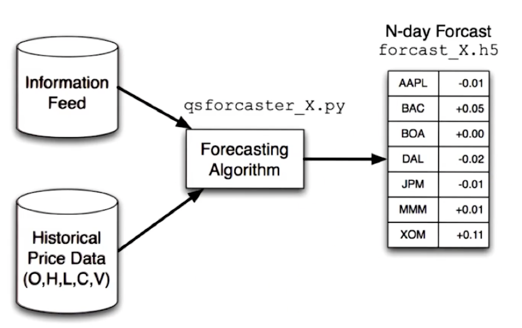
Finally, the lecture provides us with a high level overview of how the forecaster is creating the forecast leveraged by the optimizer. Again, historical data feeds into this, as well as some proprietary information feed being leveraged by the hedge fund.

Definitions

• liquid - the ease at which one can buy or sell shares within a particular holding, e.g. Stocks, ETFs. These usually have a high volume of trading.
• large cap - represented by number of shares * price of each share
• assets under management (AUM) - buzz word, how much money is being managed by the fund?
• two and twenty - 2 percent of AUM and 20 percent of the profits.

2-2: Market mechanics

This lesson covers some fundamentals of how orders are handled on the market.

What is an order?

Usually orders are sent to a stock broker and are executed on your behalf. Below is all the information that must go into a well-formed order:

• Buy or sell
• Symbol
• Number of shares
• Limit or Market
  • Market specifies that you're ok with buying or selling at the current market's price.
  • A limit specifies that you're asking for a specific price.
• Price

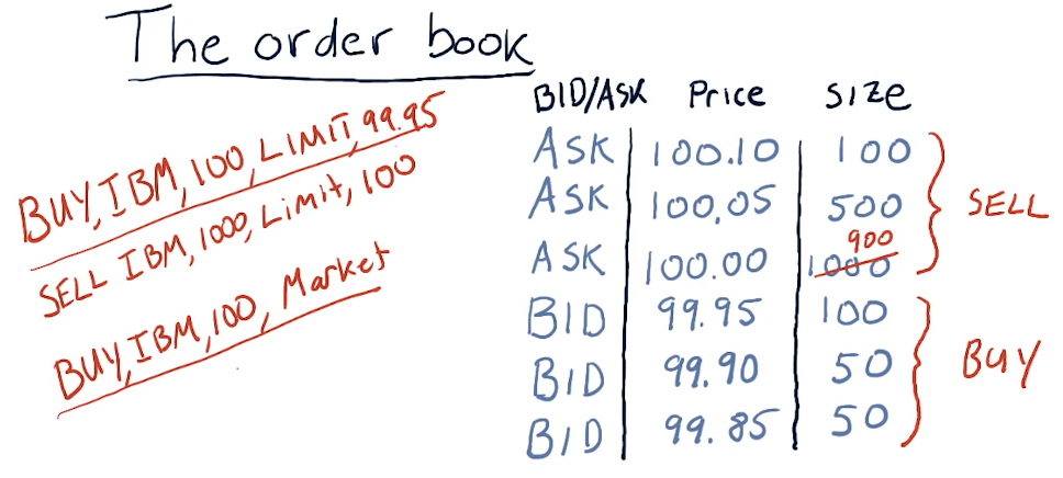
The order book

Below is a high-level overview of what a market's order book could look like during a trading day - provided by the lecture.

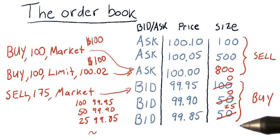
How orders affect the order book

The lecture provides a high-level overview of how the order book is affected by buy and sell orders in the market. In this example, all buy and sell orders are market orders.

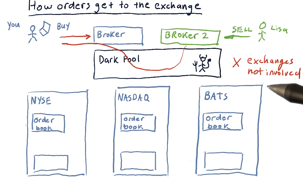
How orders get to the exchange

The lecture provides a high-level overview of how orders reach the exchange after being received by the brokers. The image below describes the existence of dark pools - I'm not sure how these are legal.

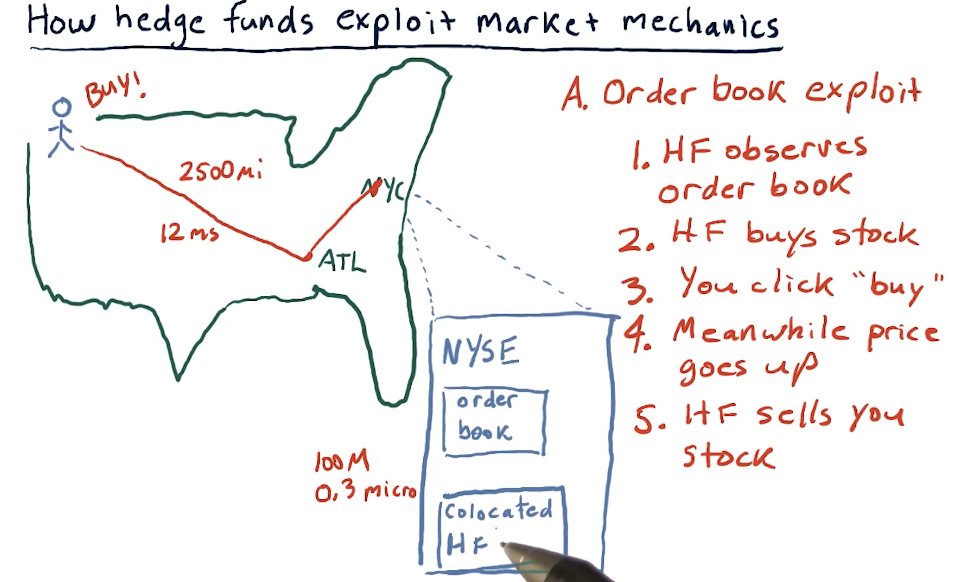
How hedge funds exploit market mechanics

Hedge funds have the ability to be co-located with the exchanges, so they can see trends in stocks faster than those who are trading remotely via brokers. Using this, they exploit the time different to buy and sell stocks at a profit. They also conduct this exploit across continents with different exchanges. A high-level overview from the lectures is provided below:

Additional order types

• Stop loss - sell the stock when it loses a certain amount of value
• Stop gain - sell the stock when it gains a certain amount of value
• Trailing stop
• Sell short - take a negative position against a stock

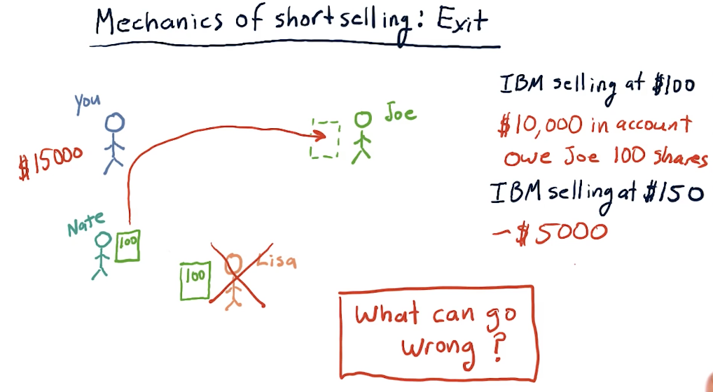
Short selling

Short selling is a strategy where we borrow stocks from someone, sell those stocks to someone looking to buy, and then when the person we borrowed from wants their stock back, we buy the stock and give the stock back as promised. What we're hoping for is that the stock decreases in value, allowing us to buy the stock at a lower price, netting us a profit.

What can go wrong?

In short selling, we can have an unlimited amount of losses. If the stock increases, we sell back at a loss, and we must give back the stock when the person we borrowed from wants their stock back.

2-3: What is a company worth?

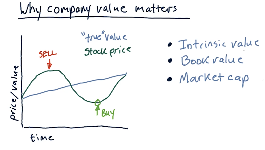
Why company value matters

A company has a true value and a stock price. The true value is not always readily apparent, and the stock value goes high or low over time, depending on trends in the market. Like always, when a stock is overvalued we want to sell and when a stock is undervalued, we want to buy.

• Intrinsic value - the value of a company as estimated by future dividends
• Book value - assets that the company owns
• Market cap - value of the stock on the market

Below is a high-level overview from the lecture of the concepts above:

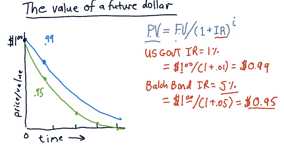
The value of a future dollar

This section of the lecture discusses the value of a future dollar - how we can calculate how much a dollar will be worth given a particular interest rate on a bond.

The equation is as follows:

• price_value = future_value / (1 + interest_rate)**years

Obviously, a dollar now is worth more than a dollar in the future. The high-level representation below displays how to calculate price value against future value given an interest rate.

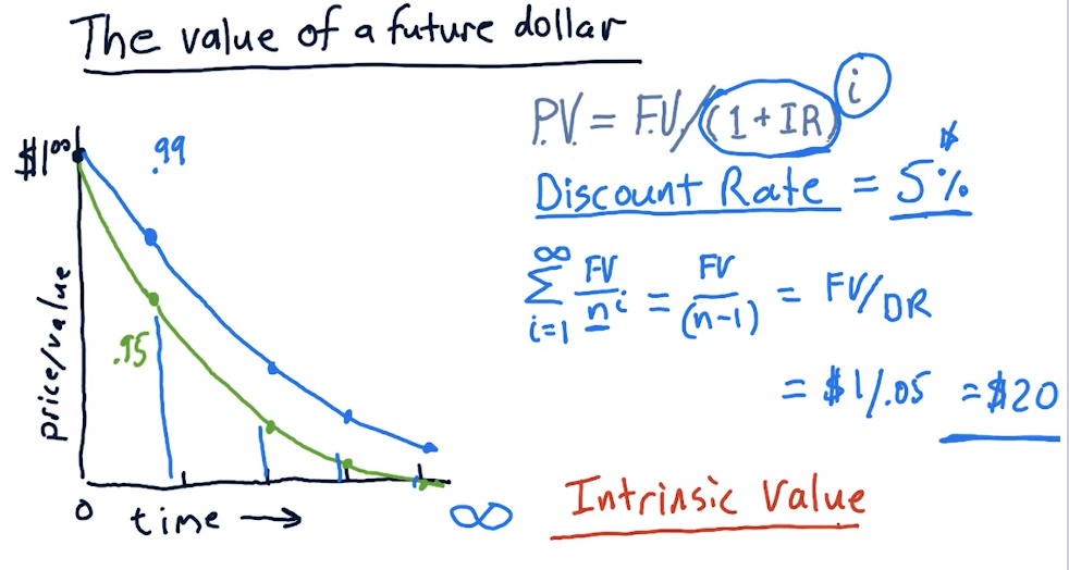
Intrinsic value

The lecture provides a breakdown on how to calculate intrinsic value, given a particular interest rate or discount rate. The equation is essentially as follows:

• intrinsic_value = future_value / discount_rate

Market capitalization

Market capitalization or market cap is simple:

• market_cap = num_shares * share_price

2-4: The capital assets pricing model (CAPM)

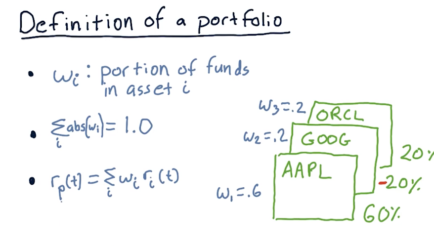
Definition of a portfolio

Before we begin talking about CAPM, the lecture first defines what constitutes a portfolio. This definition is important to effectively understand the CAPM equation.

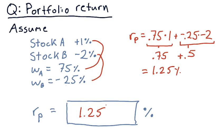
Calculating portfolio return

Below is an exercise from the lecture on calculating portfolio returns:

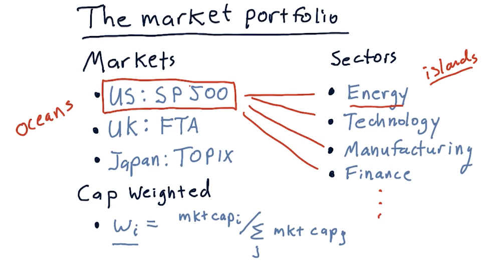
Market portfolio

The lecture provides a breakdown on what comprises a market portfolio. In this case, the discussion revolves around the SP500, comprised of the top 500 stocks in the U.S. with the highest market caps. Each stock within the portfolio is cap weighted with the following equation:

• weight = market_cap[i] / sum(market_caps)

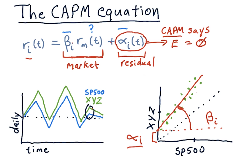
The CAPM equation

The CAPM equation is a regression equation represented as follows:

• returns[i] = (beta[i] * market_return) + alpha[i]

A definition for each variable in the CAPM equation is as follows:

• returns[i] - returns for a particular stock on a particular day
• beta[i] - the extent in which the market affects stock i
• market_return - the market's return for a particular day
• alpha[i] - residual returns unaffected by the market. The expected value E of this variable is 0.

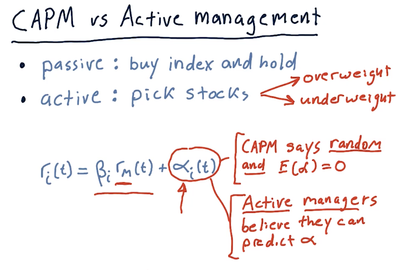
CAPM vs active management

This section of the lecture defines portfolio management strategies, passive and active. Passive portfolio management involves buying an index and holding. Passive portfolio management also assumes that alpha is random, unpredictable, and will always be an expected value of 0. Active managers of portfolios believe they can predict alpha.

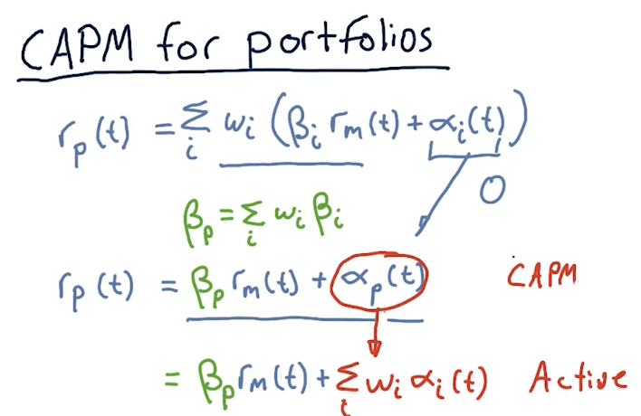
Calculating CAPM for portfolios

This section of the lectures provides us with equations to calculate the returns for an entire portfolio using CAPM. With CAPM and passive management , we can effectively assume that alpha is 0 and then we can calculate beta across all assets to arrive at a portfolio beta.

Active management strategies don't assume that alpha is 0 and will proceed to sum the alpha for all assets in the portfolio.

2-5: How hedge funds use the CAPM

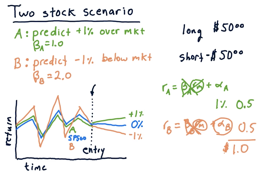
Two stock scenario

In this scenario, we've used some machine learning model to predict that a particular stock, A, will be +1% over the market and stock B will be -1% below the market. Given this, we take a long and short position to make a profit. A high-level overview from the lectures on how to calculate these returns using beta under these circumstances is provided below:

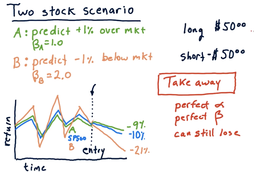
Two stock takeaways

The below snippet from the lecture reinforces that, if we're not careful with how we allocate our money, we could end up losing money taking short positions in an upward trending market, and losing money taking long positions in a downward trending market. Basically, you need to hold the right stocks with the right beta for the right market.

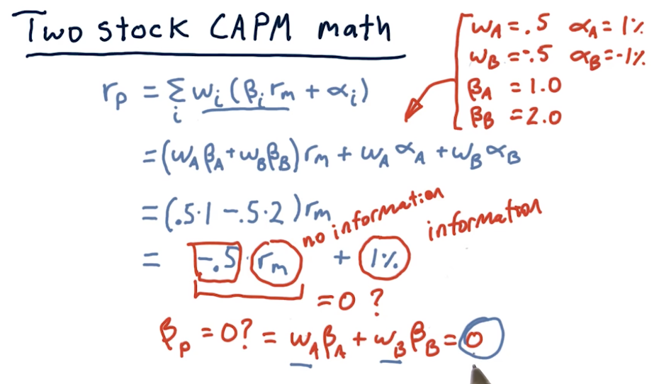
Two stock CAPM math

The lecture takes the examples provided earlier and uses CAPM to simplify the math into a regression equation. The point of this lecture is to state that we can remove market influence on our portfolio if we aim to minimize beta to 0.

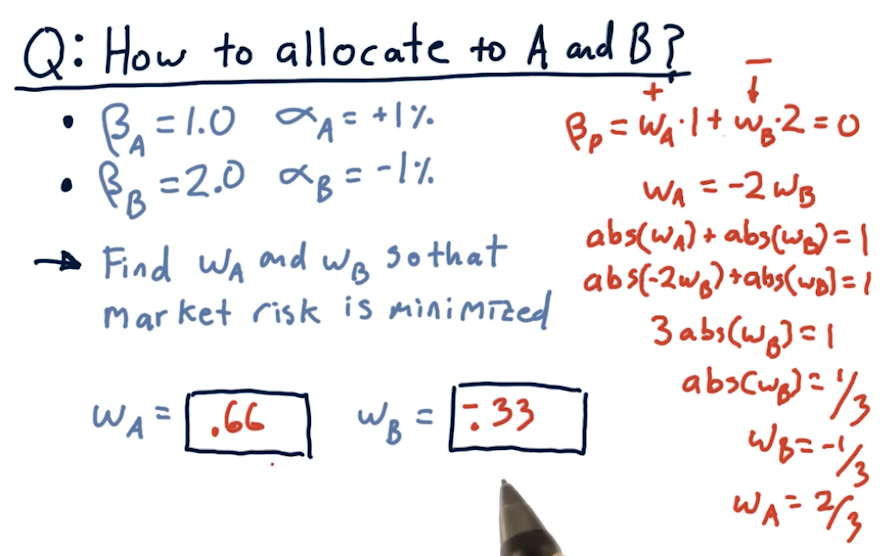
Allocations to remove risk

The lecture covers how to calculate allocations, W[i], to remove risk from a portfolio.

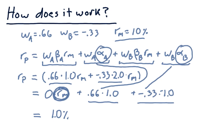
Wrapping up

The lecture covers how to calculate returns when the market has a 10% increase, given the allocations we calculated previously to remove market influence on the portfolio.

2-6: Technical analysis

There are two broad ways to choose stocks to buy or sell:

• fundamental analysis - looking at aspects of a company to estimate its value, looking to see if the price of a company is below its value
• technical analysis - looking for patterns or trends in a stock's price

Characteristics

The following are some characteristics of technical analysis:

• historical price and volume
• computing statistics called indicators
• leveraging indicators as heuristics

Why might these techniques work for technical analysis? Well, there is information to be found in the price of a stock, and heuristics work and have plenty of uses for artificial intelligence.

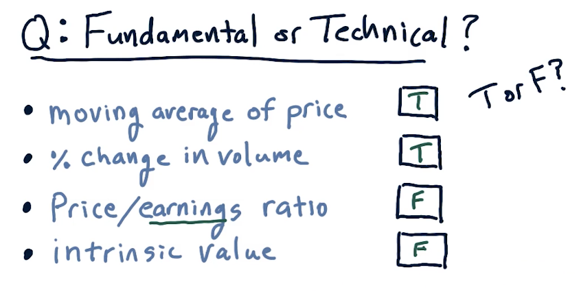
Fundamental or technical?

The following slide displays some technical and fundamental indicators:

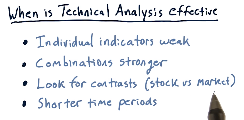
When is technical analysis effective?

The lecture provides circumstances in which technical analysis is effective:

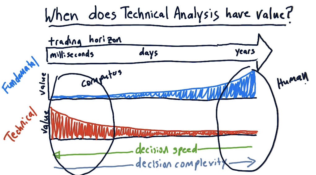
The lecture also provides a high-level breakdown of when technical analysis excels versus fundamental analysis. As we can see in the graph below, humans are best at technical analysis for long-term trading horizons, and computers are best at technical analysis in the short-term.

Good indicators

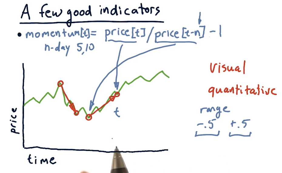
Momentum

Over X number of days, how has the price changed? It can be calculated as such:

• momentum[t] = (price[t] / price[t-n]) - 1

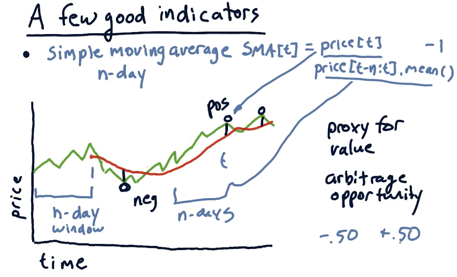
Simple moving average

Given an N day window, we calculate the average price of the stock over multiple windows. This essentially smooths out the graph of the stock. Some important events when using simple moving average are:

• The current price crosses above the simple moving average. Combined with momentum, this can by a buy signal.
• Proxy for real value. If we see diversions away from the simple moving average, we should expect to see the price return to the simple moving average. This can be used as an arbitrage opportunity.

Using simple moving average, we can also calculate point values using the following equation:

• sma[t] = (price[t] / price[t-n:t].mean()) - 1

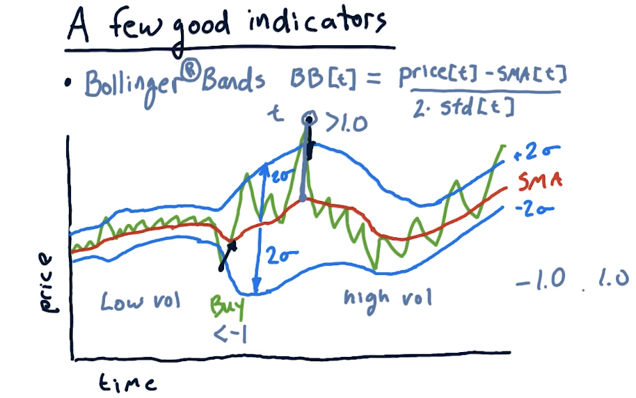
Bollinger bands

We've talked about Bollinger bands previously - these use standard deviation on the simple moving average to measure deviation for indicators. The equation to calculate a Bollinger band for a day is:

• bb[t] = (price[t] - sma[t]) / (2 * std[t])

Normalization

Plugging these indicators into a machine learning algorithm, it's quite possible that some indicators could become more influential than others. With that, we leverage normalization to provide our machine learning algorithm with indicators that maintain their original information, however, are not weighted due to their value. The equation for normalization is:

• (values - mean) / values.std()

2-7: Dealing with data

Data is obviously important for computational investing. The core data that we work with in this course is historical price and volume data.

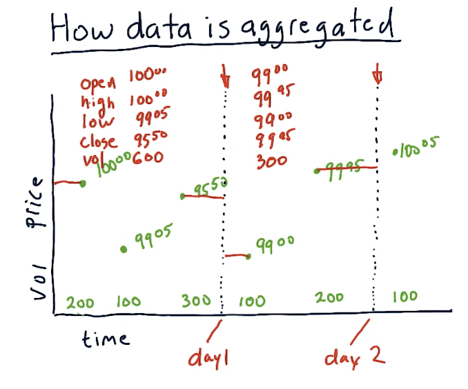
How data is aggregated

The unit of measurement for transactions is called a tick. These ticks happen at no particular time, and they can be happening across multiple exchanges. For each tick, we track the price and volume of the transaction across time. A high-level representation from the lectures is below:

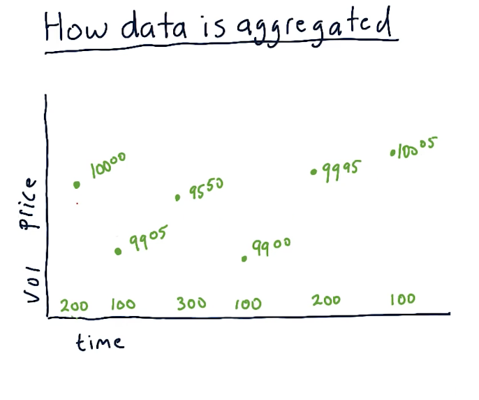
A lot of transactions occur during a trading day, and tracking every single tick requires a lot of computing and a lot of space to store the data. We can aggregate the data by only tracking the price of a specific stock during certain time slices. For this class, we'll be tracking specific metrics by day, however, with more computing you could feasibly track metrics with smaller time slices. Per time slice, we track the following metrics:

• open - the first price on the first trade
• high - the highest trade price during the time slice
• low - the lowest trade price during the time slice
• close - the last trade price during the time slice
• volume - how much of the stock was traded during the time slice

A high-level overview from the lectures is provided below:

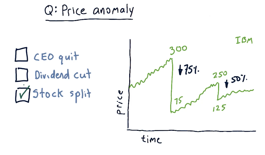
Price anomaly

A large drop in the price of shares for a given stock is called a price anomaly. A slide from the lectures is provided below. In this case, the stock experienced a stock split, cause the price to drop tremendously.

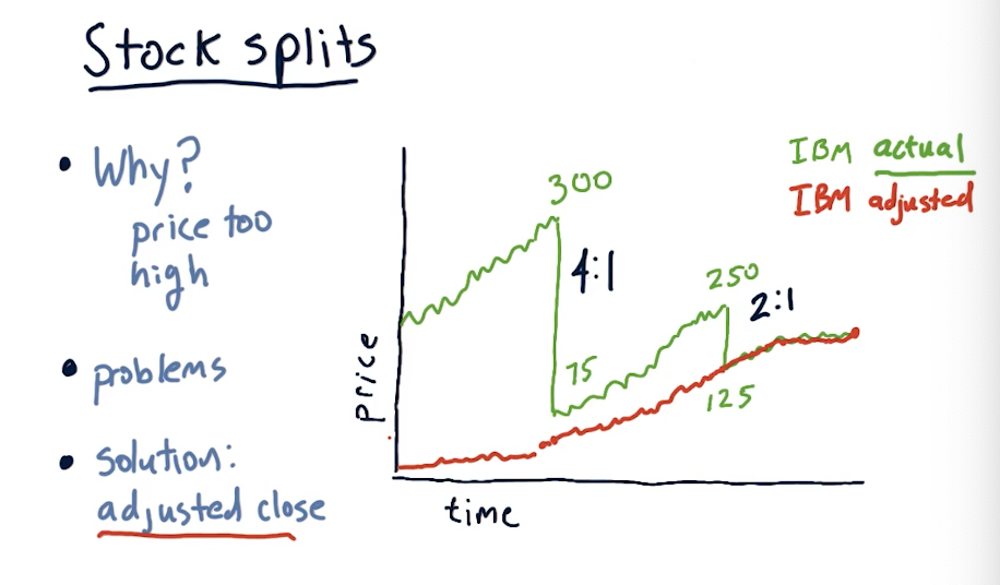
Stock splits

Why do stocks split? The most common reason is because the price is too high . Why are high prices a problem? Highly priced stocks cause them to be less liquid, making it harder to trade and buy options on the stock. High prices also make it difficult to finely tune portfolios, especially if you want to have a specific percentage of allocation for one security.

An issue with stock splits is that your machine learning model could mistake this large drop in price as an opportunity to short the stock, however, this stock isn't actually losing value - more shares are available. This is why adjusted close was created, allowing us to adjust the true price of the stock and avoid confusion due to stock splits. A slide from the lecture is provided below:

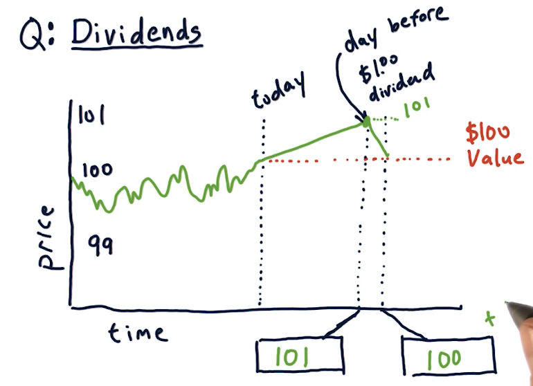
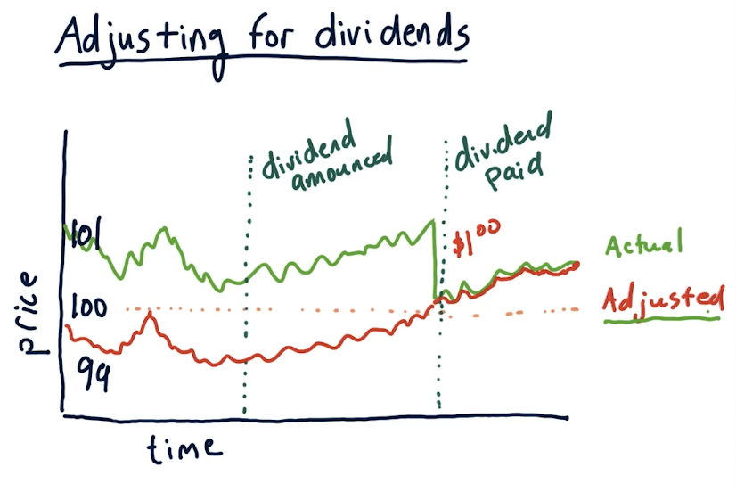
Dividends

Companies pay shareholders dividends, usually some percentage of the stock price like %1. When conducting computational trading, we'll have to account for this as the stock ticks up in price dependent upon the dividend expected to be paid out. The usual trend for a stock is that the stock rises by the amount of the dividend the day before it is processed. Immediately after that, the stock price decreases back to its original value. A slide from the lectures is below:

Adjusting for dividends

Just like stock splits, we can account for dividends by using the adjusted close price with the latest data from an exchange. A lecture from the slides demonstrating this is provided below:

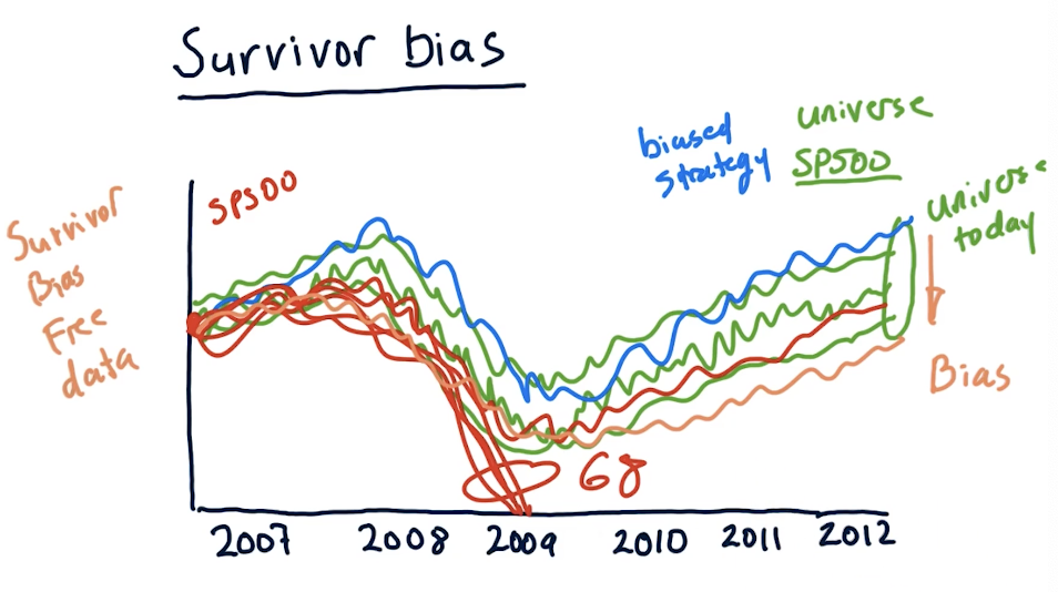
Survivor bias

Survivor bias is a built-in bias that we can encounter when analyzing our strategy over time using stocks that currently exist today. We assume that our strategy works well, but we're using data in the future, not the past. If we were to conduct the same strategy in the past, in this case in 2007, we can see that 68 stocks completely plummeted during the 2008 crash, leaving the SP500. In this case, these stocks did not survive and our strategy completely failed.

We can purchase survivor bias free data to conduct analysis of our strategy, but this is something we should always keep in mind and avoid. A slide from the lectures is provided below:

2-8: Efficient markets hypothesis

During this course, we've been operating under many assumptions. For technical analysis, we assume that there is information in historical price and volume data that we can discover and exploit in advance of the market. For fundamental analysis, we assume that fundamental data like earning can be exploited and traded upon in advance of the market. The Efficient Markets Hypothesis says we're wrong about both.

EMH assumptions

The Efficient Markets Hypothesis assumes the following:

• Large number of investors - a large number of investors are interested in the market, and are interested in leveraging technical data to make a profit from undervalued securities. Because of all of these investors, any time new information arrives the price moves.
• New information arrives randomly - new information arrives randomly at different times and rates.
• Prices adjust quickly - investors are constantly making decisions based on new information, thus the price of a stock is constantly changing due to these decisions.
• Prices reflect all available information - this is a result of the other three assumptions.

Origin of information

The following are originators of information:

• Price / volume - used for technical indicators
• Fundamental - available to everyone, usually released quarterly
• Exogenous - information about the world that affects the company
• Company insiders - reflects information that you have vs. information that people outside of the company do not have

3 forms of the EMH

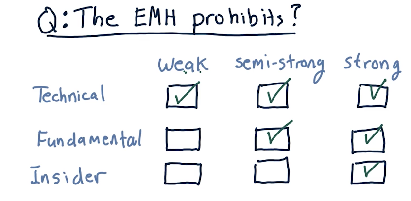
• Weak - future prices cannot be predicted by analyzing historical prices. This does leave potential room for fundamental analysis.
• Semi-strong - prices adjust rapidly to new public information. This somewhat prohibits fundamental analysis, and enables insider-information.
• Strong - prices reflect all information, public and private. This prohibits even insider information from being effective. This hypothesis suggests that the only way to make money is by holding the market portfolio.

EMH prohibition matrix

Below is a matrix breaking down which type of analysis is prohibited by different forms of the EMH:

2-9: The fundamental law of active portfolio management

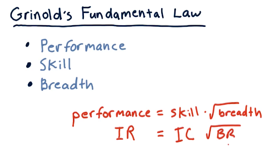
Grinold's fundamental law

This fundamental law of active portfolio management describes performance in the terms of skill and breath. These two factors create a ratio wherein you can increase your performance as an active portfolio manager by increasing your skill or you can increase the number of opportunities to test your skill. A slide from the lectures is provided below:

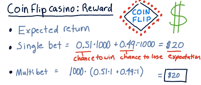
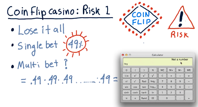
Coin flip casino

This lecture discusses some scenarios using a coin flip casino, where risk and reward are compared for different betting strategies on the flip of a coin. Fortunately for us, we know that the coin has a 0.51% chance of landing on heads.

The two betting options are:

1. Bet $1000 on one coin flip
2. Bet $1 on one-thousand coin flips

Obviously, betting $1 on one-thousand coin flips is the best option - this lecture uses this teaching point to demonstrate calculating expected value, probability, and risk via standard deviation.

Expected value

Probability

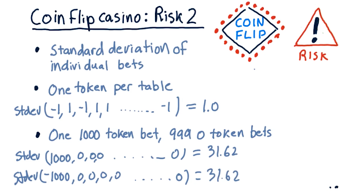
Standard deviation

Sharpe ratio

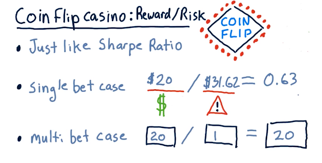
Observations

Going back to Grinold's fundamental law, if we take the sharpe ratio of the multi-bet and the single-bet and the number of bets, 1000, we encounter that this follows Grinold's fundamental law. See below for evidence from the lecture:

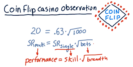
So the following are some good observations:

• Sharpe ratio grows as the square root of breadth increases.
• Sharpe ratio grows as alpha increases.

Information ratio

Information Ratio (IR) is like the sharpe ratio for excess return, alpha. The equation broken down is in the lecture slide below:

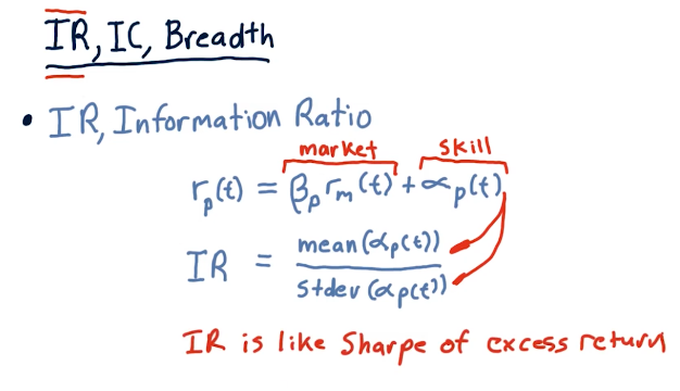
Information coefficient and breadth

Information coefficient (IC) is the correlation of an active manager's forecasts to returns. Breadth (BR) is the number of trading opportunities per year.

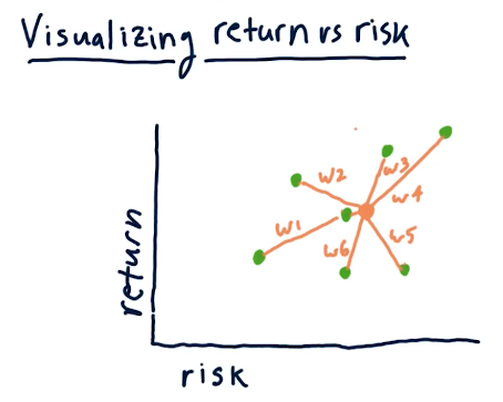
2-10: Portfolio optimization and the efficient frontier

Visualizing return vs risk

In the below slide, the professor describes how we can plot risk and return for individual stocks before allocating funds to each within our portfolio. What we can do is set the allocation for each stock differently, and find a risk/return location on a scatterplot that we're comfortable with maintaining. This is visualized in the below lecture slide:

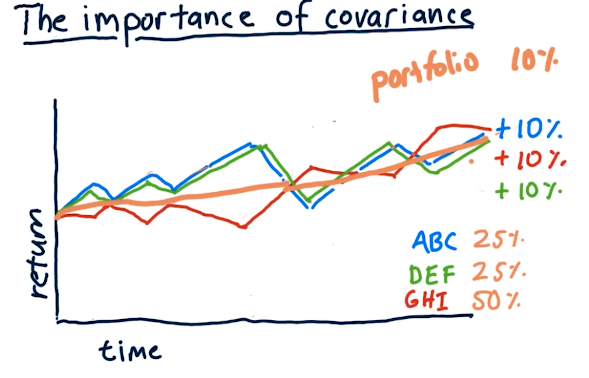
Covariance

This part of the lecture essentially covers maximizing risk while minimizing reward. In the example provided below, we allocate funds in our portfolio to securities with negative covariance, meaning when one stock goes up, the other goes down.

All of the stocks have similar returns, however, our overall portfolio encounters less risk because of the negative covariance.

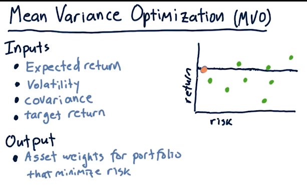
Mean Variance Optimization (MVO)

Mean Variance Optimization (MVO) is an algorithm that takes the following inputs to determine a portfolio allocation that exposes the portfolio to the least amount of risk possible and the most returns:

• expected return
• volatility
• covariance
• target return

Below is a high level overview provided by the lecture:

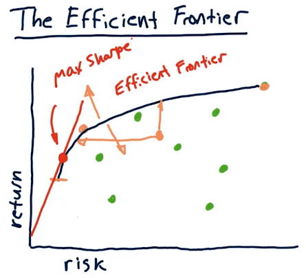
The efficient frontier

The efficient frontier is a line on our scatter plot of risk/reward security allocations - somewhere in here is a portfolio allocation for us that achieves our risk/reward tolerance. This line, the efficient frontier, is a range of optimal allocations of securities to achieve x amount of risk and y amount of return. On this line also exists a portfolio that achieves max sharpe ratio. A high level overview from the lectures is provided below:

Part 3

The following section contains my notes for Part 3 of the course "CS 7646: Machine Learning for Trading". This section of the course covers various algorithms for trading.

3-1: How machine learning is used at a hedge fund

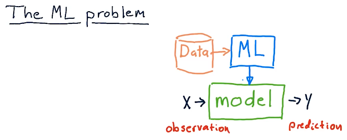
The ML problem

Plenty of hedge funds leverage machine learning models and just plain models to make predictions about the market using observation. And this essentially what a model does, machine learning or not. Provided some observation, a model produces some prediction.

In this course, we'll cover how we can process large amounts of data, provide it to a machine learning algorithm to produce a model, and use that model to make predictions from provided observations.

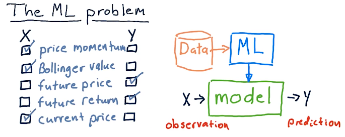
Choosing X and Y

Some examples provided by the course lecture to classify observations and predications are as follows:

• observations
  • price momentum
  • Bollinger value
  • current price
• predictions
  • future price
  • future return

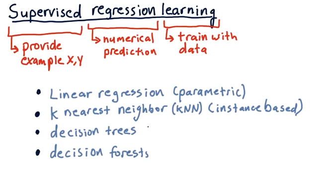
Supervised regression learning

What's the definition of supervised regression learning? Supervised means we provided an example observation and prediction. Regression means the model will be producing some numerical prediction. Learning means we train the model with some data. There are multiple algorithms to conduct supervised regression learning:

• Linear regression (parametric)
  • Leverage data to create parameters and then discards the data
• K nearest neighbor (KNN) (instance based)
  • Retains historic data and consults the data
• Decision trees
• Decision forests

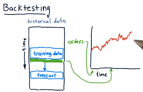
Backtesting

Backtesting is a technique wherein we utilize historical data with our machine learning algorithm and subsequent model to make predictions on events that have already happened. Using the results of our forecasting, we can make determinations as to how accurate our model is and how confident we can be in its predictions. Below is a slide from the lectures on this:

3-2: Regression

This lesson covers more in-depth topics for supervised regression learning.

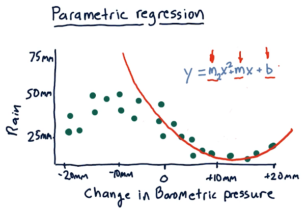
Parametric regression

Parametric regression leverages parameters in a given model to predict the outcome given some observations. In the example provided below, x is the observation of barometric pressure, the polynomial equation is the model generated by some machine learning algorithm to predict how much it's going to rain. The parameters in this case are the slope of the line, m, and the constant b.

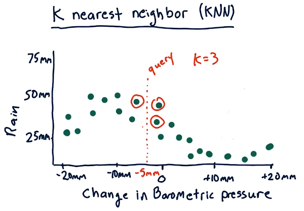
K nearest neighbor

We use the value k to select the nearest neighbor(s) for a historical data point to make a prediction. The slides from the lecture, below, demonstrate how, for a given query, we use this algorithm to select 3 of our nearest neighbors to predict the amount of rain given historical data. We take the mean of the nearest neighbors to generate our prediction.

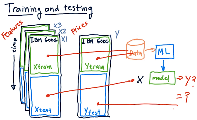
Training and testing

This section of the lecture covers how we treat our data for training and testing. Our training data should be separate from our testing data. The training data should be used with some machine learning algorithm, parametric or KNN, to generate a model. Once the model is generated, we can then use the testing data to make predictions.

3-3: Assessing a learning algorithm

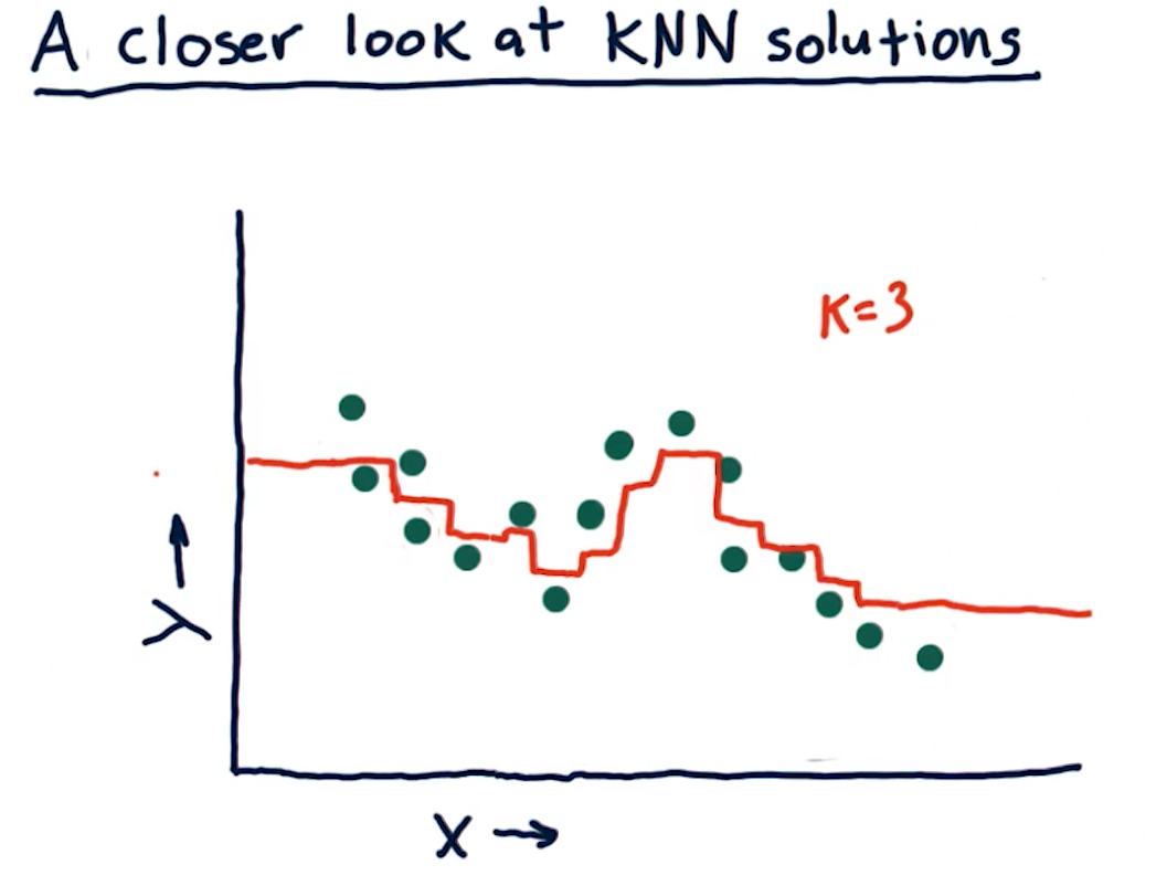
A closer look at KNN solutions

This section of the lecture just reviews KKN solutions and how trend lines can be generated from them by using the KNN algorithm. In the example from the lectures below, we see that we're taking the mean value for k nodes at some point x, y and drawing the entry at that location. The greatest drawback of this method is that, on the edges, we receive straight lines because of the back fill and forward fill of data:

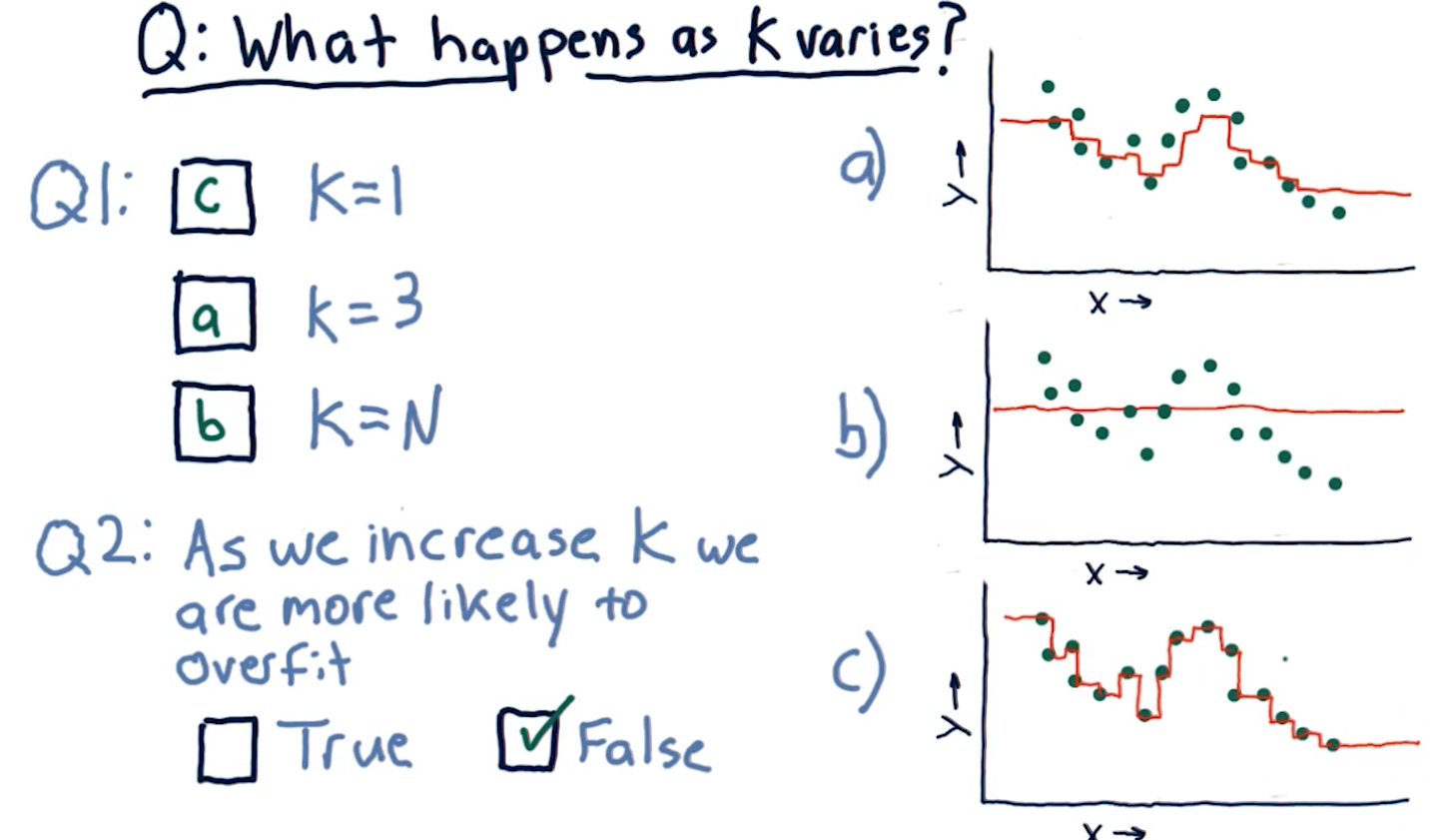
What happens as K varies?

When k approaches N number of entries, we see that the graph drawn provides us less information - it essentially becomes a straight line for some sets of data. In contrast, a k value of 1 provides us with a line that is basically discrete. The final question this section in the lecture asks is: "As we increase K we are more likely to overfit?". The answer is false, as k increases the line drawn fits less of the data.

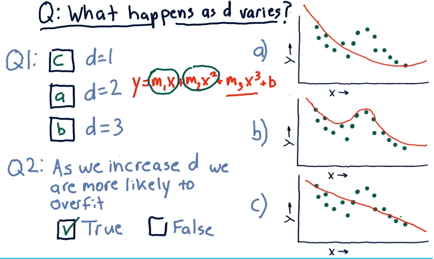
What happens as D varies?

D in this case represents a parametric model's number of parameters: x1, x2, x3, and so on. This section of the lecture presents the same question: "As we increase D are we more likely to overfit?". The answer is true, as we increase the number of parameters in a parametric model, the line in our graph becomes more complex and fits the data in our dot-graph more closely.

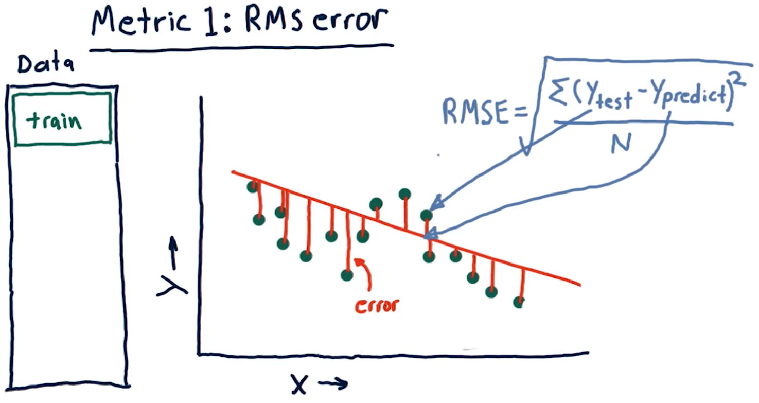
Metric 1: Root Mean Squared error

When assessing a learning algorithm, we need to be able to derive some metrics from the model's prediction. These metrics provide us with the ability to tune our algorithms, and subsequently our models. This section talks about root mean squared (RMS) error. How this metric is derived is provided by the formula in the screenshot, below:

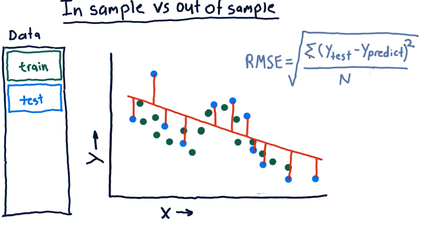
Out of sample error

Out of sample error is the RMS of our model's evaluation of the test data instead of the training data. A representation of this concept from the lecture is provided below:

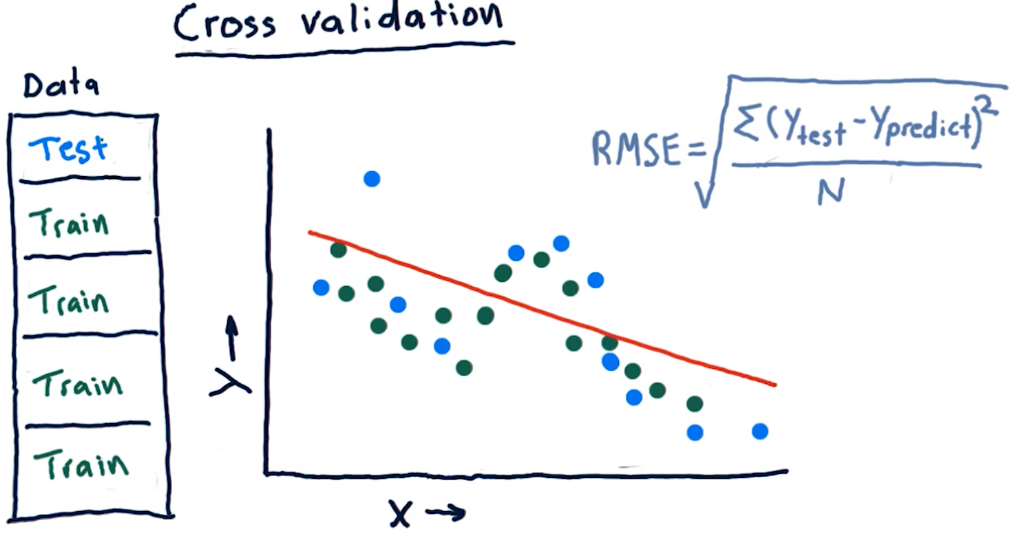
Cross validation

Researchers categorize trials for a learning algorithm as the following procedure:

• Select a set of data
• Slice the data into train data and test data
• Conduct training on the data marked for training
• Conduct testing on the data marked for testing
• Calculate the RMS error for the model's performance on both the training and the testing data

We conduct cross validation by running a series of trials on the same data, slicing the data into proportionate chunks and alternating which chunks are used for training and which chunks are used for testing. Each alternation of testing and training data is considered a trial.

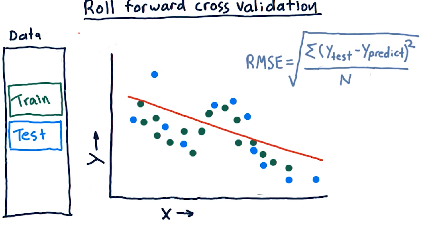
Roll forward cross validation

Cross validation is a useful technique, however, it poses some limitations for creating machine learning models for trading. Specifically, it allows the model to peek into the future, providing optimistic predictions that aren't necessarily useful for trading.

To avoid this, we ensure that train data is, chronologically, always before the test data. This is called roll forward cross validation and it helps us avoid the issue discussed in the previous paragraph.

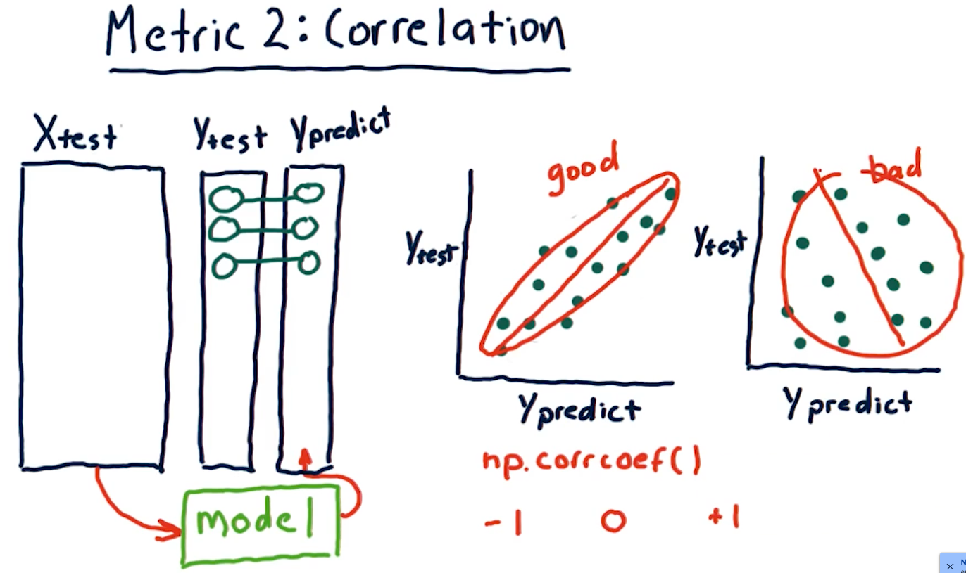
Metric 2: Correlation

Another metric, correlation, provides us with information as to how often our predictions are correct in comparison with some test data. Given a set of test data, x, y with x being an event and y being the result, our model should produce another set of data x, y1 where y1 is the model's prediction.

To measure correlation, we graph y vs y1. Our correlation is good if our resulting graph is linear and increases as y and y1 increases. Our correlation is bad if there doesn't seem to be any resulting linear graph.

The NumPy method np.corrcoef() provides us with a measure of correlation for two sets of data with the following ranges:

• 1 denotes that the data is heavily correlated
• -1 denotes an inverse correlation
• 0 denotes no correlation
• The values provided by this method can range between the values of 1 and -1.

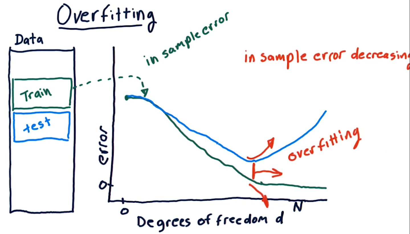
Overfitting

Overfitting is a phenomenon wherein our out of sample error begins to increase as our degrees of freedom (the number of a parameters in our parametric algorithm) begins to increase. Our in sample error decreases to 0 as our degrees D approaches N number of samples. As shown in the diagram below, however, on test data, due to overfitting, our out of sample error begins to increase as D approaches N.

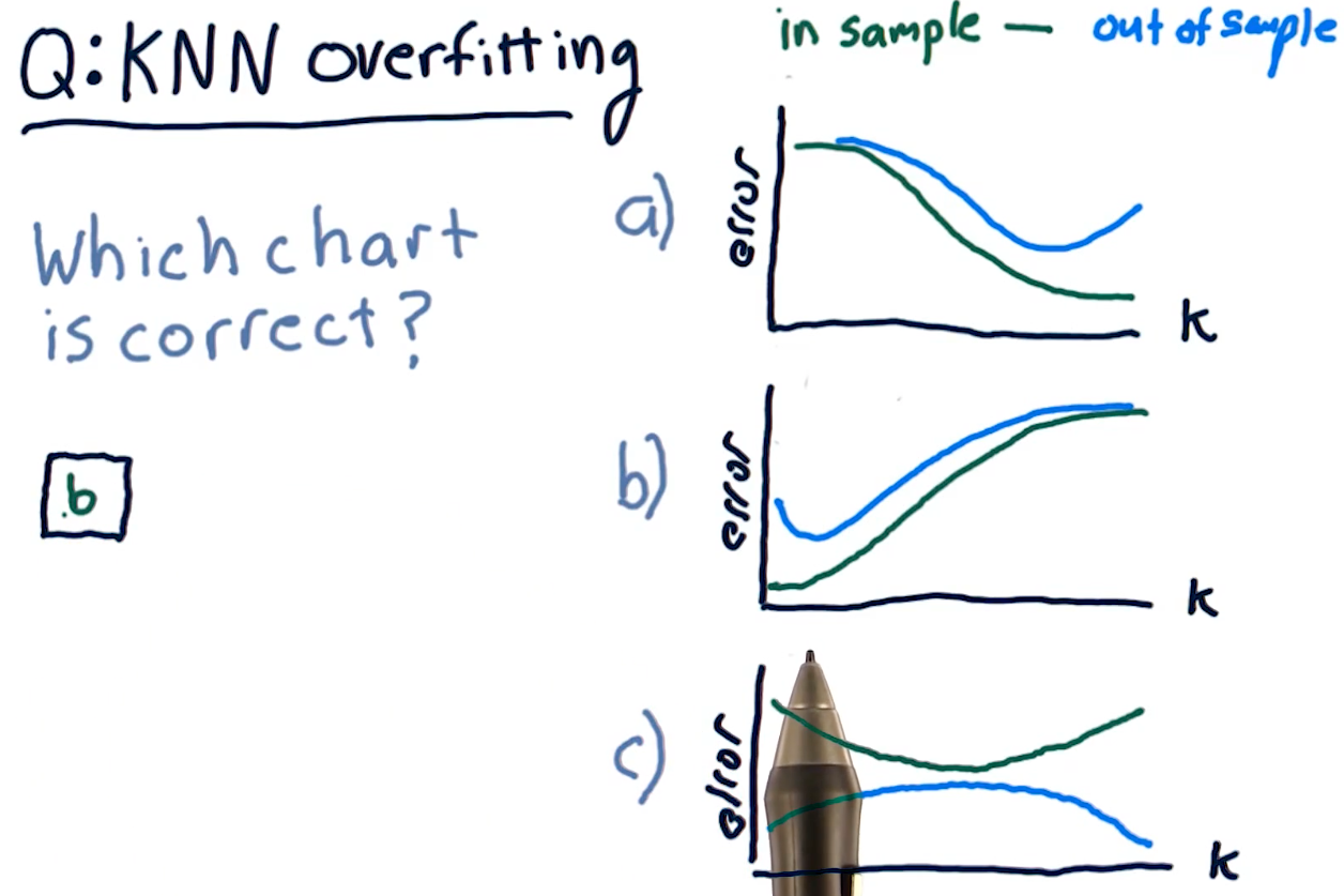
KNN overfitting

Overfitting for KNN algorithms behaves a bit differently. Because a KNN-produced line becomes too general as K approaches N, both our out of sample error and in sample error increase as K approaches N. The sweet spot for K is somewhere where out of sample error decreases a significant amount at the cost of in sample error.

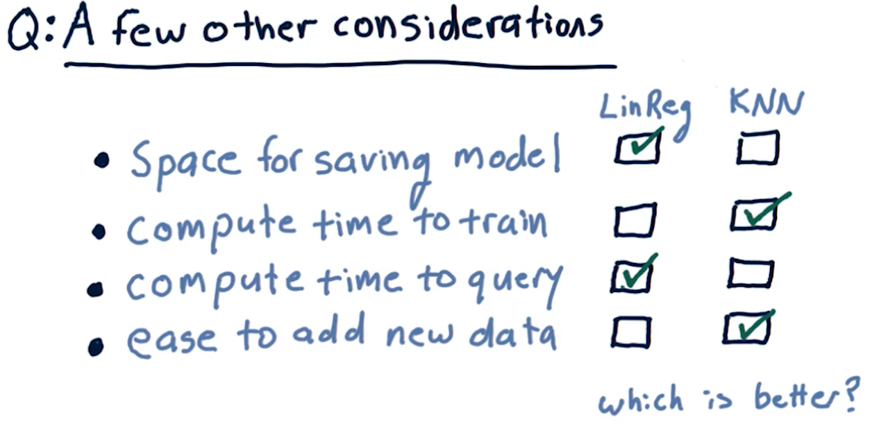
Final considerations

The following diagram outlines pros and cons of each learning algorithm with respect to compute time, query time, etc.

3-4: Ensemble learners - bagging and boosting

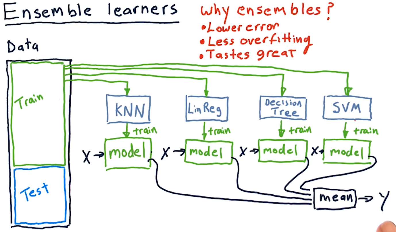
Ensemble learners

Creating an ensemble of learners essentially means that we leverage multiple different machine learning algorithms to produce a series of different models. For regression-based learning, we provide each produced model an x and take the mean of their y responses. Why use ensembles? Ensembles provide:

• Lower error
• Less overfitting
• Removal of algorithmic bias

A diagram representing this concept is provided below:

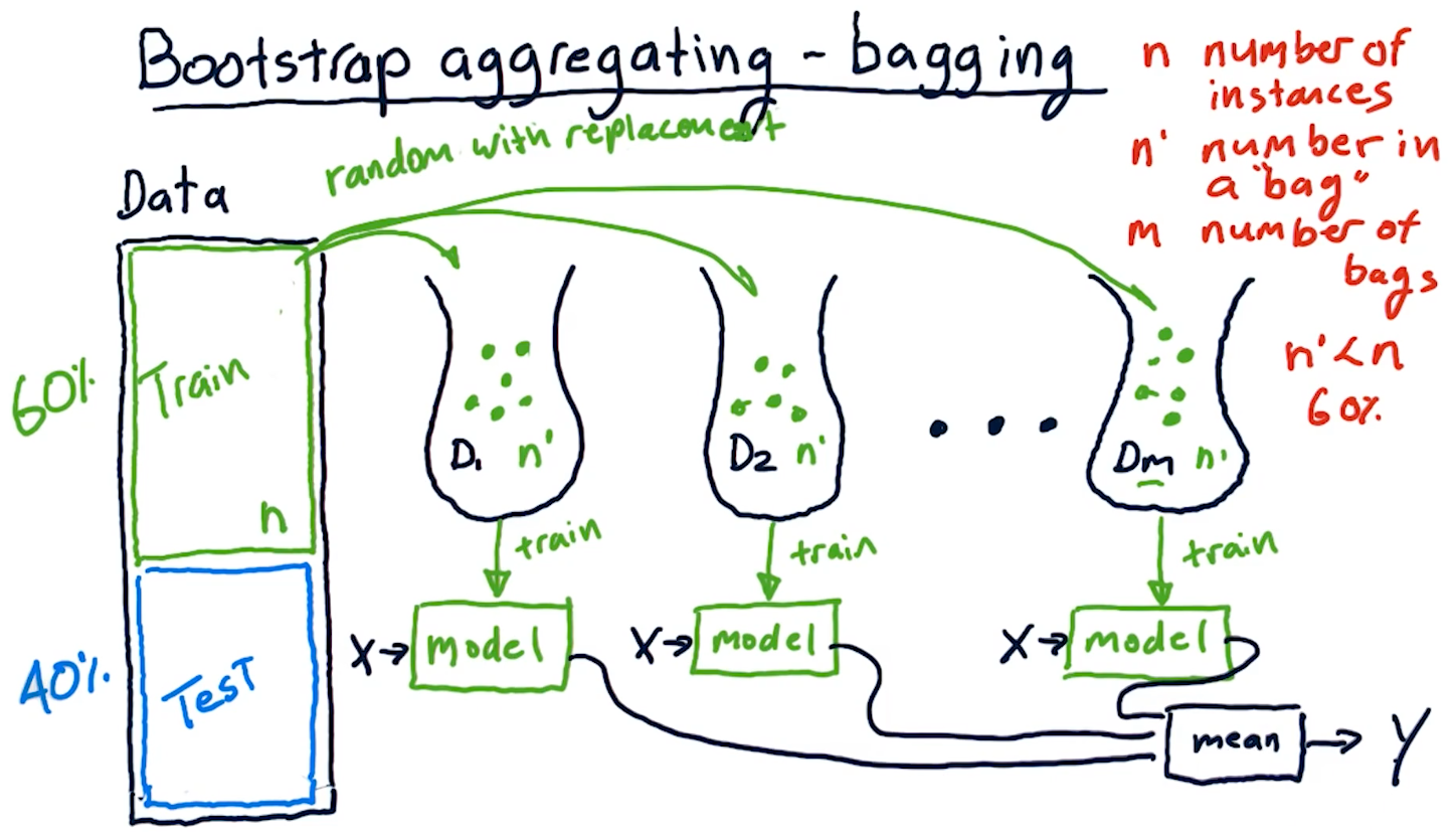
Bootstrap aggregating-bagging

Bagging is a method of creating an ensemble of learners, however, we utilize the same learning algorithm to create m number of bags and models. What is a bag? A bag is a set of data derived from the original training data for a learning algorithm, with up to n' items. n' will always be some subset of n - usually 60%. The n' items selected from the original data are random with replacement - we can have duplicate items selected from the original data.

After we create our m bags with n' number of items, we use these bags to train our models with the same learning algorithm. Like our ensemble before, we take the mean of the models' predictions to generate our y.

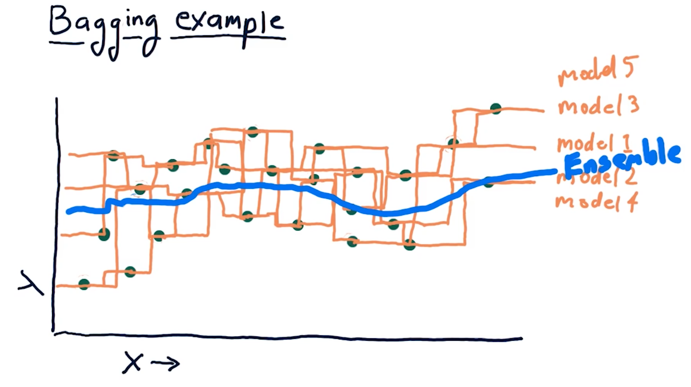
Bagging example

The example diagram provided below demonstrates how an ensemble of 1NN-generated models, using a different subset of random data for each model, generates a much more smooth predictive line than a single 1NN-generated model. Recall that 1NN-generated models overfit the data, however, if we combine these overfit models into an ensemble, the mean prediction provides better correlation with the data.

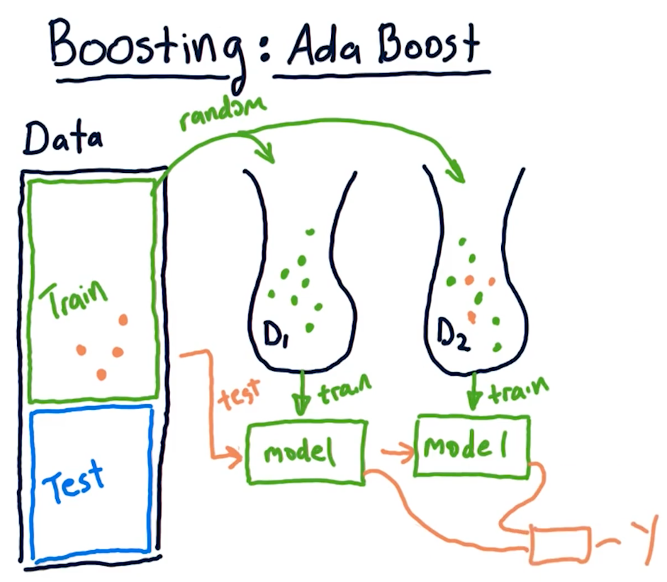
Boosting: adaptive boost

Boosting is a technique similar to bagging, however, it aims to provide weight to particular sections of data in the training data set that may be poorly predicted. Boosting conducts the following actions:

• Select random values from n to generate a bag m of n' values
• Train a model and test the model against the original data within n
• Identify x, y predictions from this model that performed poorly
• Generate new model with n' values that are weighted toward n values with poor predictions
• Train a model with the weighted data and generate more x, y predictions
• Calculate the mean of y with the old and new models
• Iterate over this procedure m times

3-5: Reinforcement learning

Reinforcement learners provide policies on which actions to take. Recently we've only been focused on regression tree learners.

The RL problem

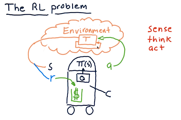
The professor breaks down reinforcement learning in the terms of robotics, since he's originally a roboticist. These concepts can also be applied to stock trading, but the pieces of the puzzle are as follows:

• reinforcement learning follows a sense, think, act cycle.
• We have some policy called pi that receives the state of the environment, S.
  • pi generates some action, A.
  • This action has some affect on the environment.
• Changes are made to the environment based upon our actions, and then we sense again to acquire the environment's state S.
• Ultimately, we receive some reward R from our actions on the environment, and we want our reinforcement learning to maximize that reward.
• Finally, our algorithm Q interprets what actions generate a state that ends up in a reward, and uses this to update the pi policy.

All of these concepts can also be applied to a Q-learning robot that generates orders in the stock market. Please find below a high-level overview from the course:

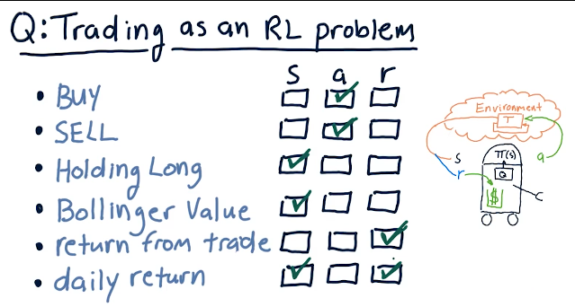
Trading as an RL problem

The professor provides us with a quiz to break down different actions, states, and rewards in regards to trading:

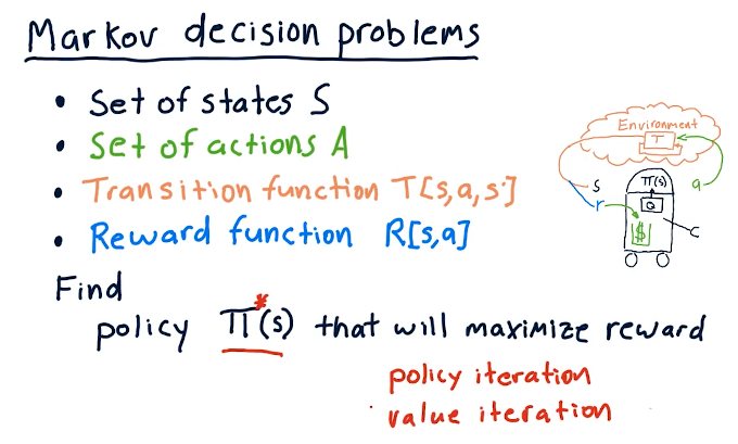
Markov decision problems

Pretty much covers the previous sections, however, we discuss transition functions where we identify states S, some action A, and then we find probabilities to end up in state S prime. Our transition function must sum all probabilities for this three-dimensional data structure to 1.0. We also have a reward function that identifies that some state S also provides us with a reward by executing action A.

So the purpose of solving this problem is to find policies pi that interpret S to maximize reward. How we do this is via:

• policy iteration
• value iteration

Unknown transitions and rewards

Experience tuples are sets of data that relate a state, an action, a state prime after the action occurs, and a reward. As we continue to encounter new situations, this data structure increases in size with the number of experiences.

We can leverage this data in two ways to conduct reinforcement learning:

• model-based
  • build a model using transition functions and reward functions
  • conduct value or policy iteration
• model-free
  • this involves q-learning where we inspect the data as a whole

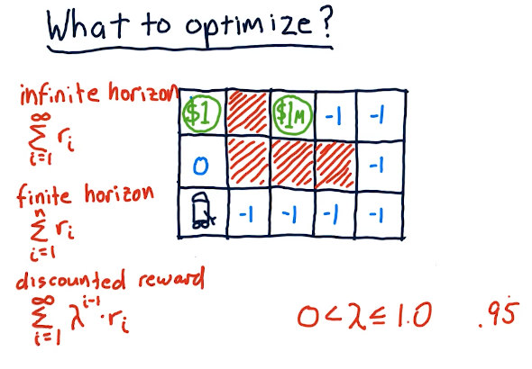
What to optimize?

The professor discusses the different types of reward given the amount of time we have to acquire that reward - our horizon. In the slide below, the robot searches for a reward - obviously the $1 reward is more immediate while the $1M reward is harder to reach.

What we use in Q-learning is the discounted reward, modified by gamma as the horizon approaches infinity. Gamma can effectively be our interest rate and, as we see here, it effectively devalues our reward as time goes on. This is all to say that money today is worth more than money tomorrow.

3-6: Q-learning

Q-learning is a model-less approach. It does not care about or use models of transition functions like T or rewards functions like R. Q-learning builds a table of utility values, or Q-values, at each step to select the best action based on what it has learned so far. The best thing about Q-learning is it is guaranteed to provide an optimal policy.

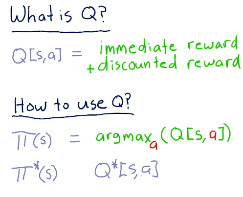
What is Q?

Q is similar to the other functions like T and R, however, it represents the immediate reward and discounted reward for an action taken in a specific state. Q is not greedy, and considers the discounted reward - so what happens today and tomorrow.

We use Q to generate a policy, pi, by finding the maximized argument value for action to maximize the Q value. Eventually, we'll have an optimal policy.

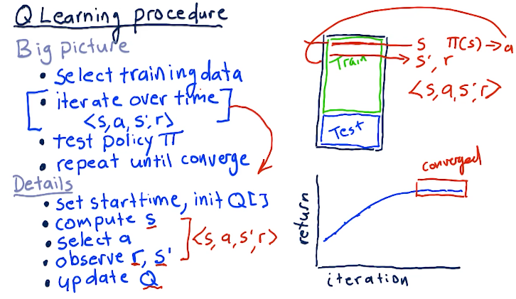
Q-learning procedure

A series of things occurs when training our Q-learning model and generating our Q table:

• First, we select our training data
• We iterate over this time-series data
  • We set a start time and initialize our Q table
  • We compute the starting state S given the inputs
  • We select our action A
  • We observe our end state S' and our reward
  • We update Q based on the outcomes
• Once we've generated our Q table, we test the policy, pi against testing data
• Finally, we repeat until convergence, resulting in no further improvements

A high-level overview of these concepts is provided below:

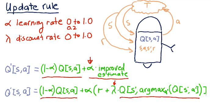
Update rule

One of the most important parts of Q-learning is the update rule. We can break it down into simpler terms wherein our new Q table, Q prime, is equal to our old Q table times 1 minus alpha, the learning rate, plus alpha times our reward plus gamma times the Q table value derived from alpha prime of our next decision to reach S prime. The writeup for the update rule equation is provided in the lecture slide below:

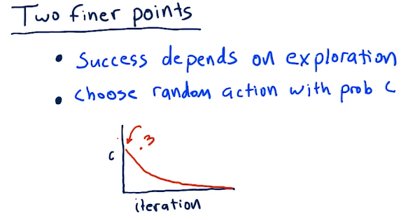
Two finer points

Q-learning is successful when we explore, and we can do that by taking random actions. We can choose random actions with probability of C. So as we begin to learn, we start out with C's probability of us choosing a random action to be pretty high. As we begin to learn more, our actions become less random.

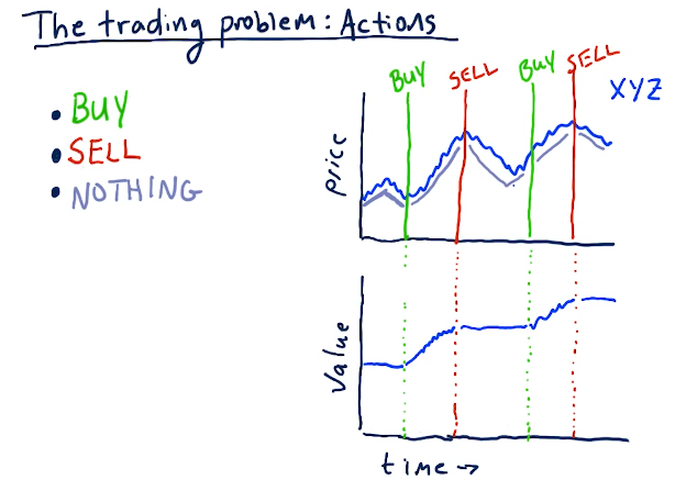
Actions

For our stock trading Q-learner, the following are some actions that can be taken to transition to different states:

• Buy
• Sell
• Nothing

Below is an example from the lectures:

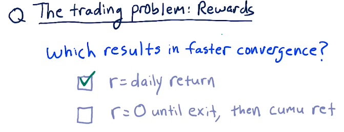
Rewards

Daily returns for a reward signal to the Q-learner allows the learner to converge must faster than a cumulative return.

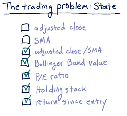
State

Below are some good factors for state to be used during Q-learning:

Creating the state

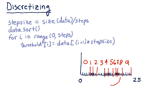
In order for us to create the state, we have to translate all of our factors into discrete integers. Some algorithm will conduct this, and then we'll finally combine our factors into one number. Below is a lecture from the slides:

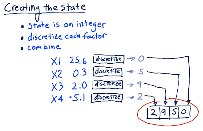
Discretizing

Below is a quick breakdown from the lecture on how to discretize our data:

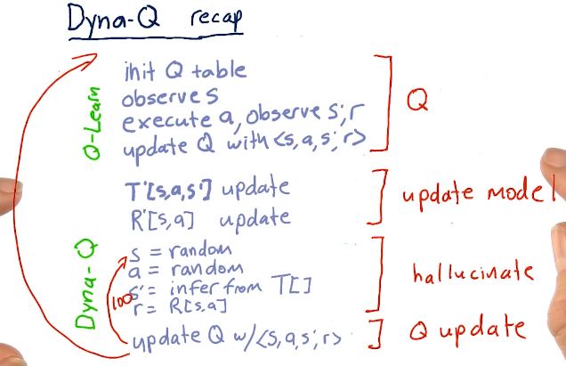
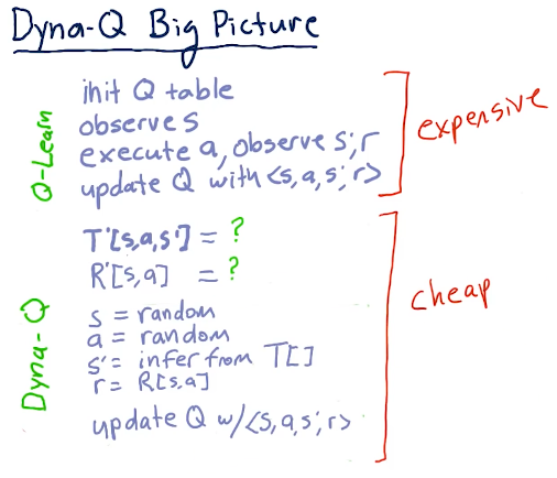
3-7: Dyna

The issue with Q-learning is you have to execute real trades to receive feedback from the real world in order to converge while learning. Rich Sutton invented Dyna to solve this problem. Dyna builds models of T, the transition matrix, and R, the reward matrix, and then, after each interaction with the real world, hallucinates many additions interactions - usually a few hundred.

Dyna-Q big picture

With Dyna-Q, we have a Q table that is influenced by real-world actions, states, and rewards. After this expensive operation is done, we take those findings and update our backend Dyna-Q T and R models. We conduct an iteration 100 times, learning about the information we just received from the real world and this is used to update our Q-learner used for real-world solutions.

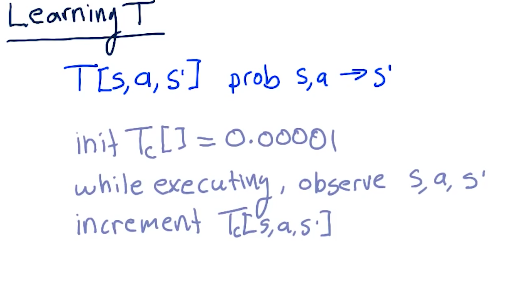
Learning T

We start of with T being equal to 0.00001. While executing, if we observe a state of S transitioning to S prime due to some action, we increment the counter for that respecting T location.

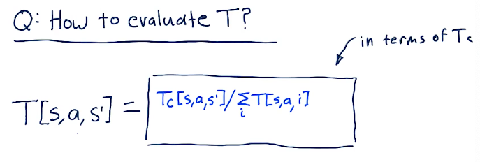
Evaluating T

We evaluate T by determining the probability we'll end up here based upon taking this action and arriving at this state, using historical data. Essentially, we'll take Tc, number of times we've been at this state due to action at S, and we'll divide that by the sum of the number of times we've been at this state and have taken the same action and arrived at a different or the same state. This essentially just iterates through all states related to this action.

This gives us the probability of arriving at state S prime. Equation from the lecture is provided below:

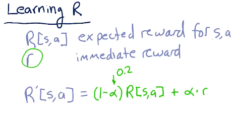
Learning R

R is the expected reward for a state and action and r is the immediate reward we experienced for this state and action. R prime is the update we make for this R after receiving new observations, and it's similar to updating Q. Below is the equation for this:

Recap

Below is a high-level recap from the lectures: