Welcome

This notebook contains my personal notes for CS6290: High Performance Computer Architecture offered at the Georgia Institute of Technology. A summary of the course follows:

This course covers modern computer architecture, including branch prediction, out-of-order instruction execution, cache optimizations, multi-level caches, memory and storage, cache coherence and consistency, and multi- and many-core processors.

Course links

• https://omscs.gatech.edu/cs-6290-high-performance-computer-architecture
• https://ebookcentral-proquest-com.prx.library.gatech.edu/lib/gatech/detail.action?docID=787253

Introduction

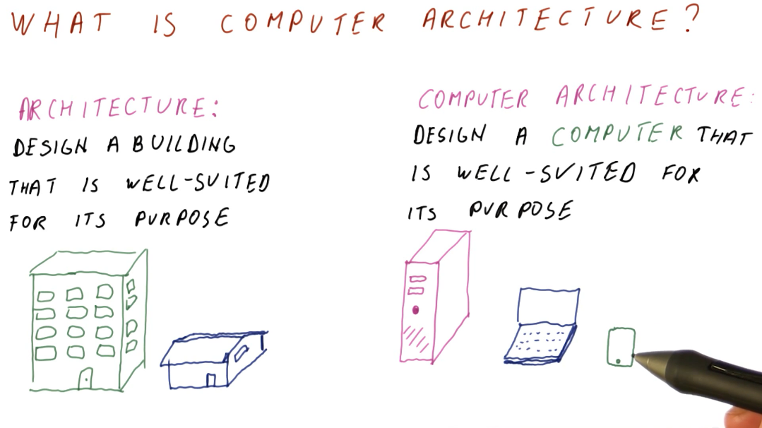
What is computer architecture?

We can think of computer architecture similar to how architecture is considered for building. Buildings are designed to be well-suited for a specific purpose. The same can be said of computers, as we design different computers for different purposes. Some examples are desktop computers, laptops, and cellphones; they all have different purposes and require different computer architectures.

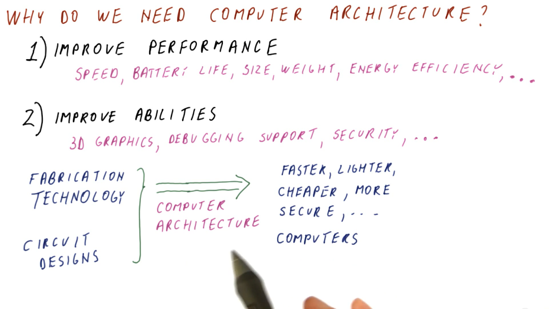
Why do we need computer architecture?

1. To improve performance based upon some specific measure. These measures could include:

• Speed
• Battery life
• Size
• Weight
• Energy efficiency, etc.

2. To improve the abilities provided by a computer. These abilities could include:

• 3D graphics
• Debugging support
• Security, etc.

The first need for computer architecture is about making computers cheaper, faster, smaller, etc. while the second need is based around making new things possible/providing new functionality. Computer architecture utilizes discoveries in fabrication technology and circuit design to achieve the goals stated above.

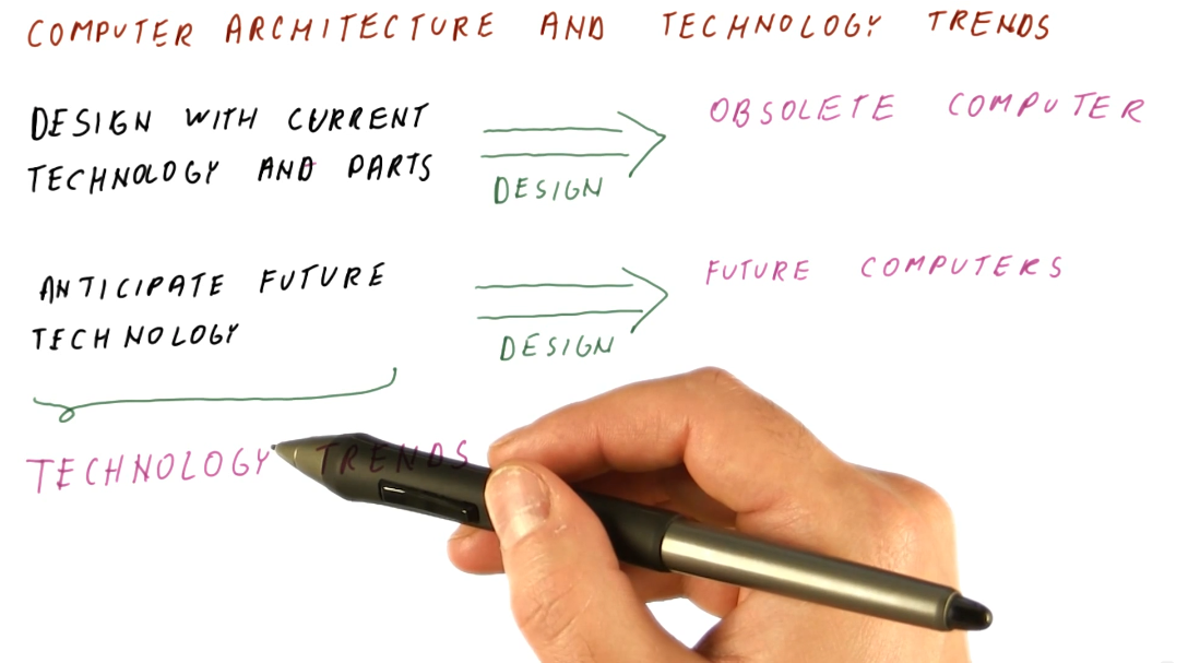
Computer architecture and technology trends

Computer architecture is about building future computers. The progress in computer manufacturing technology is fast. We shouldn't design a new computer with current technology and parts. By the time we've designed our new computer, it's obsolete and using old technology. We need to track technology trends in order to predict what's available in the future, allowing us to better design a new computer using these new technologies.

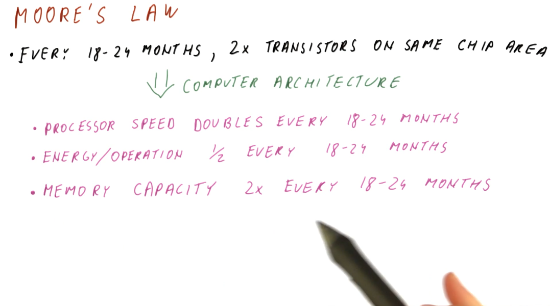
Moore's law

Moore's law provides a good starting point for predicting what future computers will look like based upon what is currently available today. As computer architects, we can use these predictions to guide our expectations of what technologies will be available for use when designing future computers. Below is a high-level summary of Moore's law:

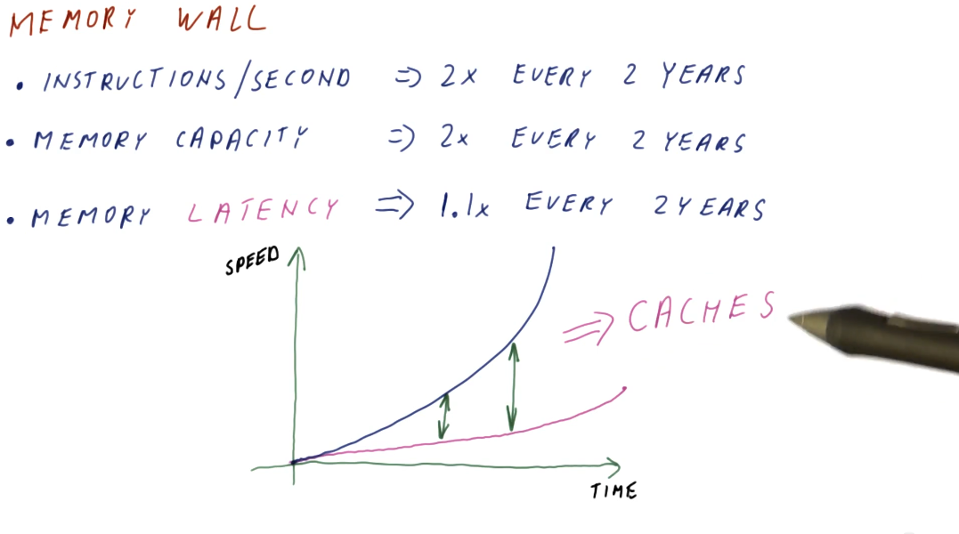
The memory wall

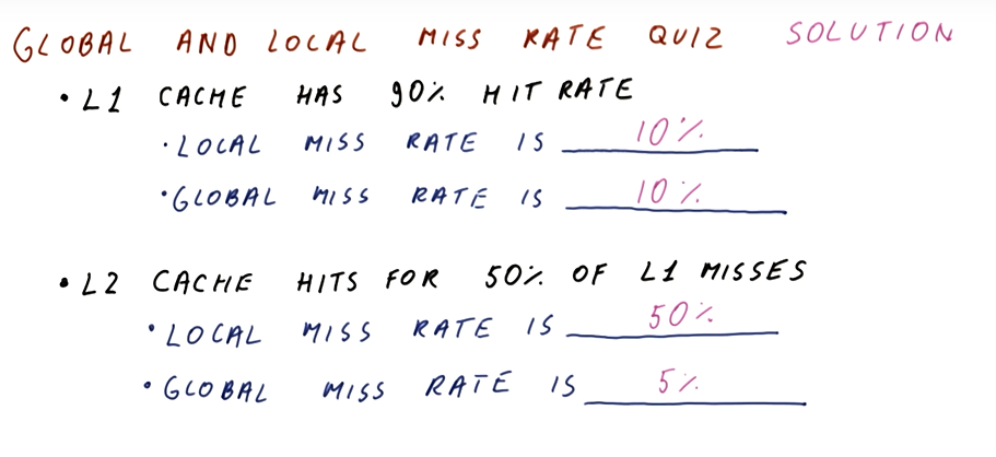
Processor speed doubles almost every two years, while memory capacity also experiences the same phenomenon. Memory latency, however, has not kept pace with processor speed and memory capacity. This is what's called the memory wall and, in order to mitigate these differences in speed when processors need to access memory, we have been using caches to close that gap. Caches can be thought of as a series of stairs for memory access speed, and cache misses are the base of the staircase with the slowest memory access speed possible. A high-level illustration of the memory wall trend is provided below:

Power consumption

There are two kinds of power that a processor consumes:

• Dynamic (active) power - consumed by activity in a circuit
• Static power - consumed when powered on but idle

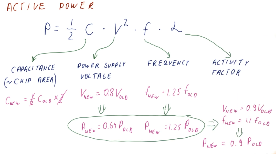
Active power

Below is an illustrative representation of the equation for calculating active power consumption by a processor. The representation also displays how we can calculate the change in active power consumption when a different chip configuration is used, and if voltage and chip frequency are changed. An explanation of each variable in the active power equation follows:

• capacitance - roughly proportional to chip area / larger chips will have more capacitance
• voltage - quadratic relationship between voltage and power consumption
• frequency - clock frequency (GHz) of a processor
• alpha - activity factor (percentage of processor transistors active for any given clock cycle)

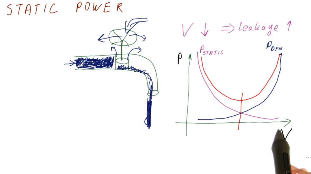
Static power

Static power is power consumed while the processor is idle. Some of this is due to the voltage being too low to prevent transistors from leaking/wasting energy, but it can also come from other sources as well. Below is a high-level representation identifying the relationship between static and active power as voltage increases or decreases in the circuit. This representation also identifies that there is some optimal voltage settings for circuits to avoid utilize too much power in bot the active and static states.

Fabrication cost and yield

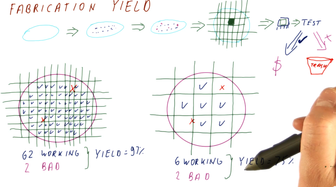
The cost to manufacture and convert silicone wafers to useable computer chips is pretty much static. We, primarily, have to account for chip yield when a silicone wafer is divided into a number computer chips - some of these chips can have defects while others work fine. Below is high-level representation of the silicone wafer to computer chip manufacturing process, and how the yield is derived based upon the number of defects in wafer versus the number of chips extracted from a wafer.

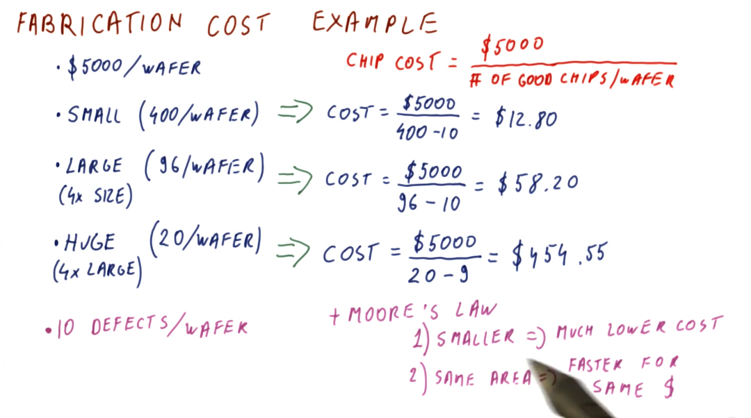
Below is an example of how we can calculate the fabrication cost per chip based upon chip size. Smaller chips cost less to manufacture, while larger chips cost the most. Smaller chips, over time according to Moore's Law, will be able to do more for less as we are able to fit smaller transistors onto the chips. Larger chips will be able to remain the same size and cost, however, they will be faster overall due to Moore's Law.

References

1. Lesson 1 Notes

Metrics and Evaluation

This lesson covers latency and throughput, two metrics used to measure computer performance.

Performance

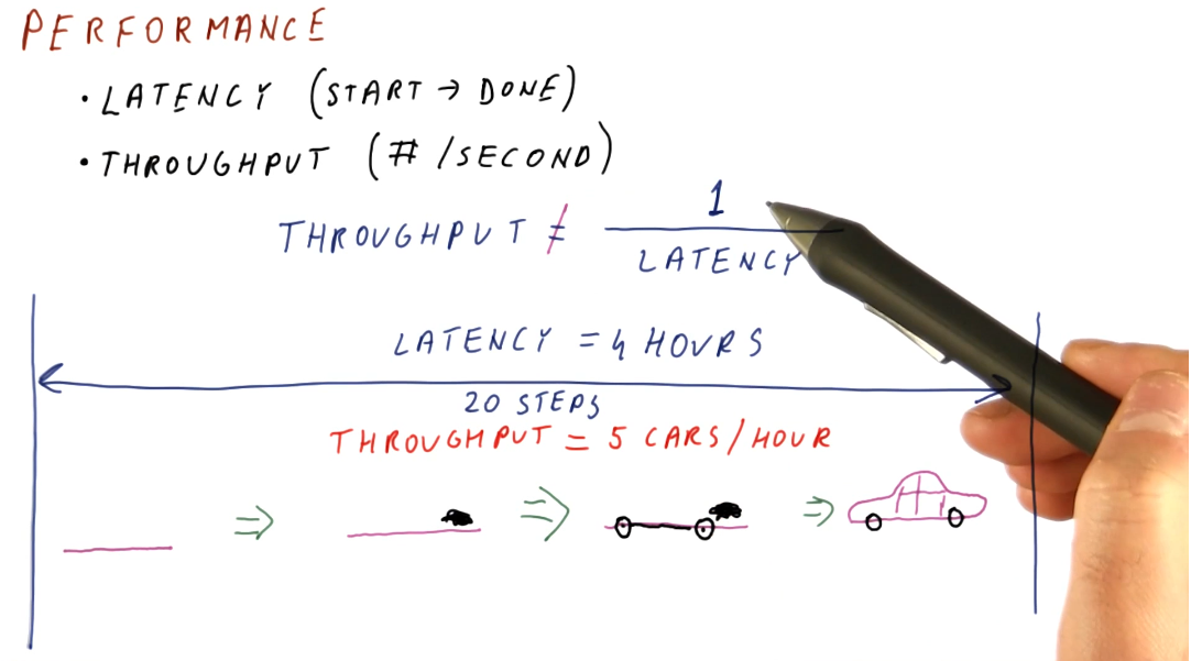
• Latency - the total time it takes for an operation to complete, from start to finish.
• Throughput - not the inverse of latency; because operations can take place concurrently within a pipeline, this can be thought of as the number of operations completed per unit measure of time.

Below is a high-level representation of this concept.

Comparing performance

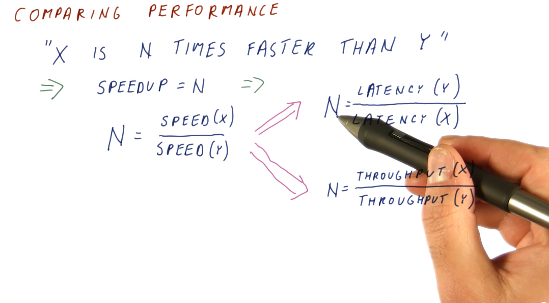
Knowing how to measure performance, we can now compare the performance of two systems using our metrics. We want to be able to make a definitive statement about the speedup of a system in comparison to another system, basically stating that system x is faster than system y. We can compute this with both latency and throughput, however, our equations are slightly different. Below is an image showing us the equations for computing speedup using our two metrics.

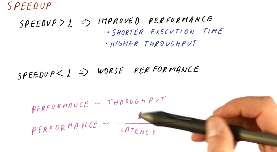
Speedup

A speedup value larger than 1 means we have improved performance. With improved performance, we achieve higher throughput and shorter execution time. A speedup less than 1 means that we have worse performance. When computing speedup, we need to remember that performance is directly proportional to throughput and performance has an inverse relationship with latency.

Measuring performance

What workload do we use to measure performance of different systems? We can't use an actual user workload because:

• Many different users use computers in many different ways with many different programs.
• One workload will not be representative of all users.
• How are we supposed to acquire the workload data?

In order to solve this issue, we use benchmark workloads.

Benchmarks

Benchmarks are programs and input data that users and organizations have agreed upon for use in performance measurements. Usually, we don't have just one benchmark program but a benchmark suite consisting of multiple programs and input data. Each program within a benchmark suite is representative of a type of application.

Types of benchmarks

So what types of benchmarks are commonly used to measure performance? We have:

• Real applications

  • Most representative of real workloads.
  • Also the most difficult to setup on new machines. Our testing environment likely doesn't have an operating system, hardware, graphics processors, etc.

• Kernels

  • The most time consuming portions of an application, usually a loop of some sort. We've isolated these processing intensive sections of code to test our machine. Usually good for testing prototypes.

• Synthetic benchmarks

  • Behave similar to kernels but are simpler to compile. We utilize these benchmarks when testing early prototypes of a machine. Usually good for design studies.

• Peak performance

  • Performance that's not based on running against actual code. The theoretical highest number of instructions per second. Usually good for marketing.

Benchmark standard

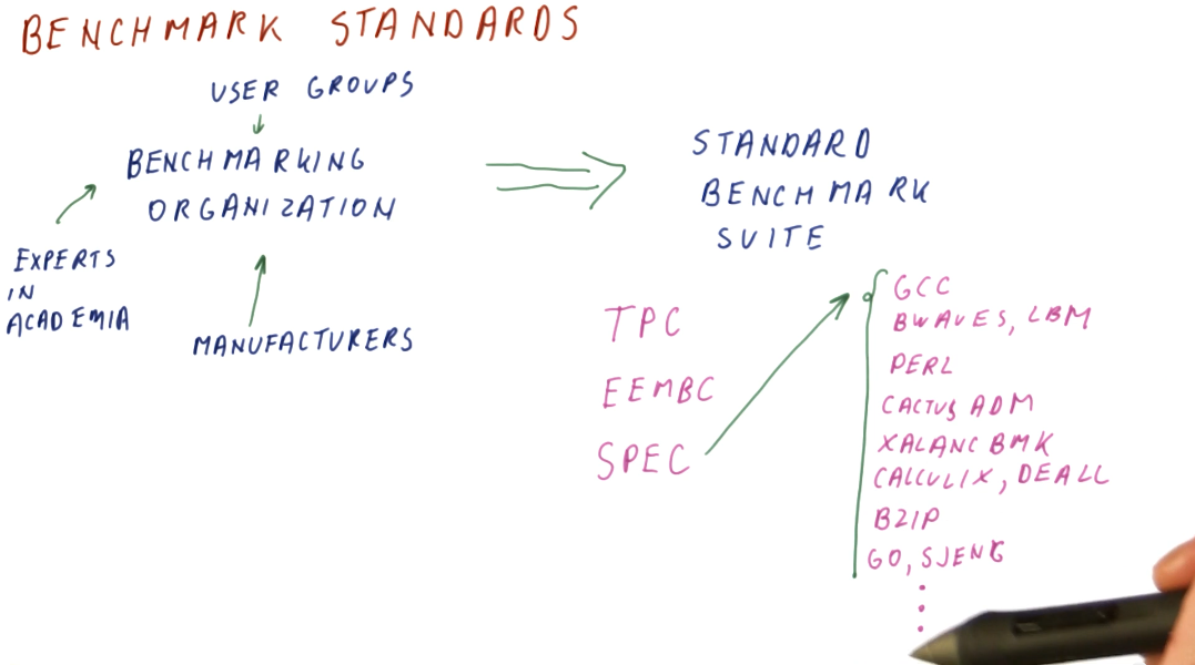
So how are benchmark suites created? Who makes them and what are the standards? There exist standards organizations that receive input from manufacturers, user groups, and experts in academia and these organizations produce standard benchmark suites. Some well known standard benchmark suites are:

• TPC - Benchmarks used for databases, web servers, data mining, and other transaction processing. [1]
• EEMBC - Used for embedded processing. [2]
• SPEC - Used to evaluate engineering work stations and raw processors. SPEC encompasses a large set of workloads, trying to cover a variety of uses for processors in high performance systems. A breakdown of these workloads is in the image below. [3]

Summarizing performance

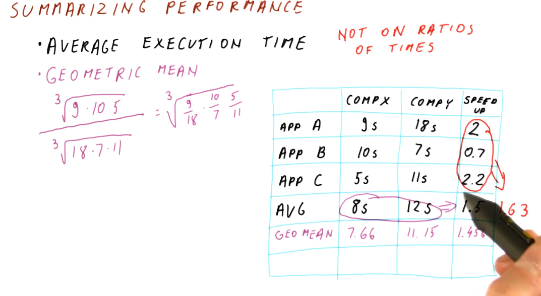
To summarize performance, we are looking for the average execution time. A demonstration on how to calculate this is shown below. We should refrain from averaging the speedups for each application tested - averaging ratios will not provide useable data to summarize performance. In order to acquire the average speedup, we need to use the geometric mean for the execution times of each computer.

Iron Law of performance

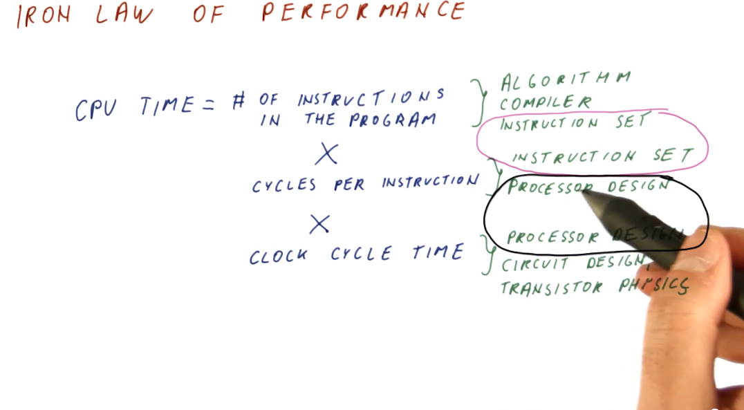
Processor time (CPU time) can be expressed as: (instructions/program) * (cycles/instruction) * (seconds/cycles)

So why do we think about these components of processor time instead of just measuring processor time directly? These three components allow us to think about the different aspects of computer architecture.

• (instructions/program) - influenced by the algorithm used to create the program, the compiler used to interpret and generate the program, and the instruction set being used.
• (cycles/instruction) - influenced by the instruction set being used, and the processor design.
• (seconds/cycle) - influenced by the processor design, circuit design, and transistor physics.

Computer architecture primarily focuses on instruction set and processor design, and good designs of these two aspects attempts to balance their effects on CPU time.

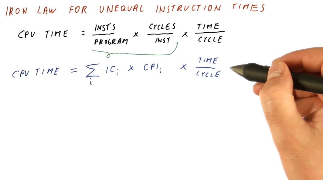
Iron Law for unequal instruction times

It's pretty simple to calculate CPU times when we assume that all instructions for a program will take the same amount of cycles to execute. This isn't always the case, however. We need to be able to sum all the cycles for each type of instruction before we multiply this with our time per cycle. Below is a representation of this concept, showing us how to calculate a more realistic CPU time.

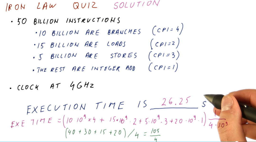
Below is an example problem in which we calculate the sum of cycles for a program in order to determine the CPU time.

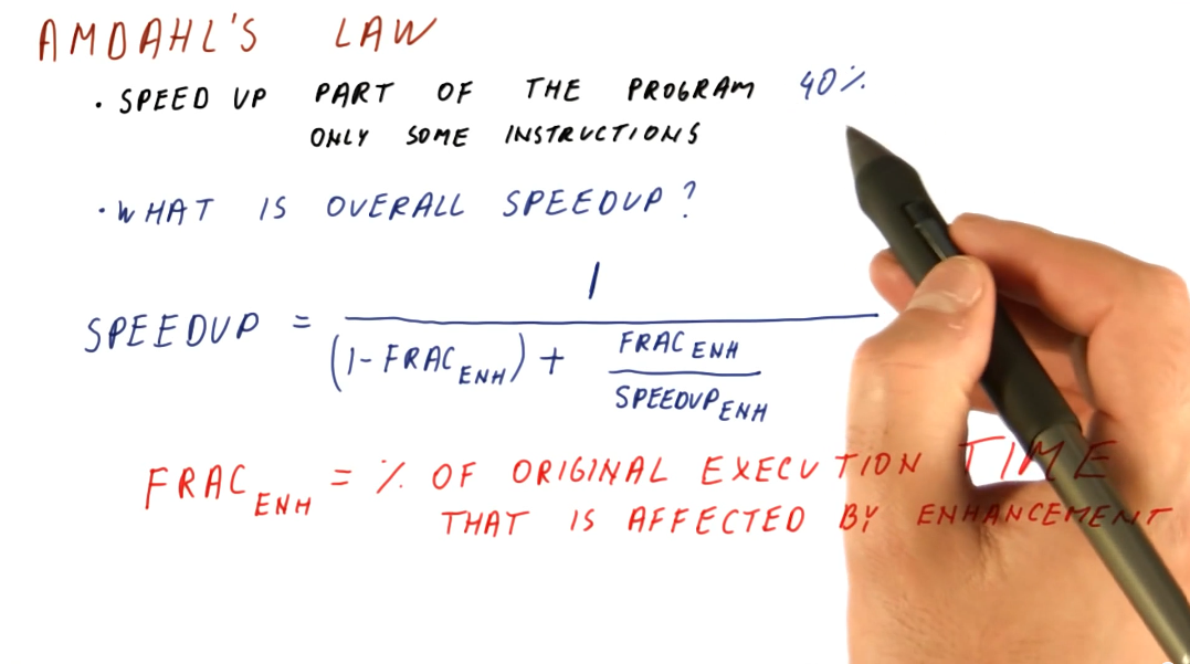
Amdahl's Law

This law is useful when we need to calculate the overall speedup of the entire program, but we only enhanced a fraction of the program. Below is an image that attempts to explain the equation for Amdahl's Law, a description of each variable in the equation is provided:

• (1 - frac_enh) - the fraction of the program that wasn't enhanced.
• frac_enh - the fraction of the program that was enhanced.
• speedup_enh - the speedup achieved due to the enhancement.

It's very important to understand that frac_enh is a percentage of the original execution time that is affected by the enhancement.

Implications

It's important to aim for enhancements that achieve a speedup on a larger percentage of execution time for a program. This is demonstrated mathematically below.

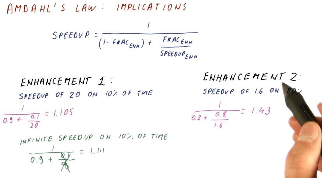
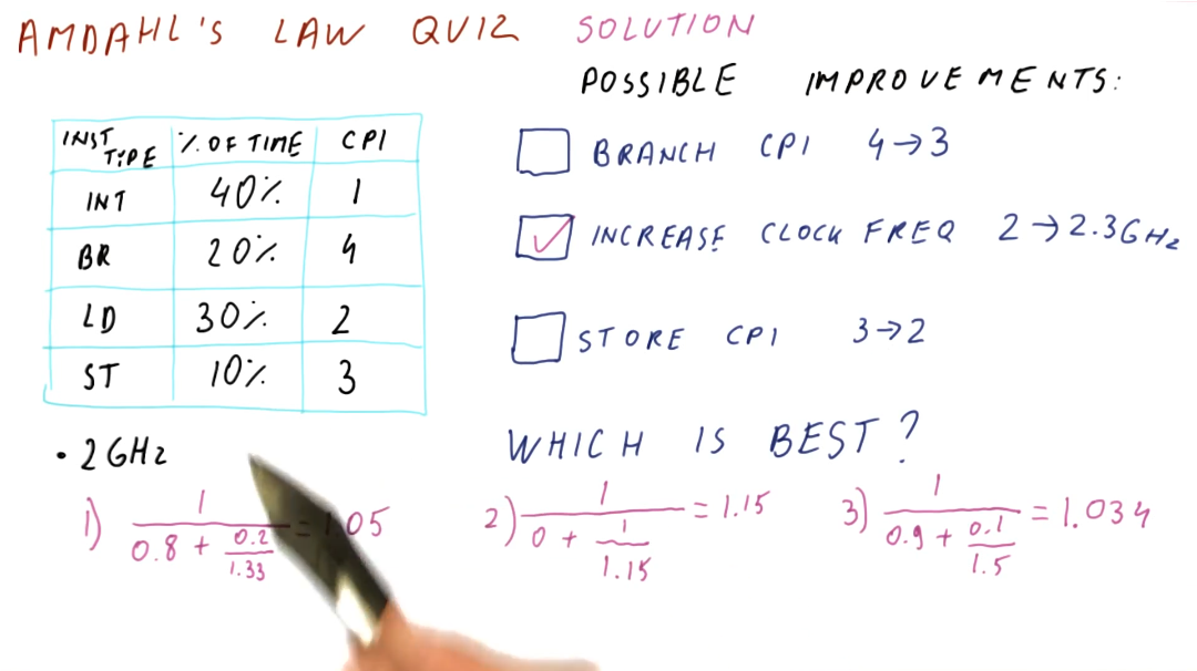
Below is an example of how to use Amdahl's Law to compare multiple possible improvements.

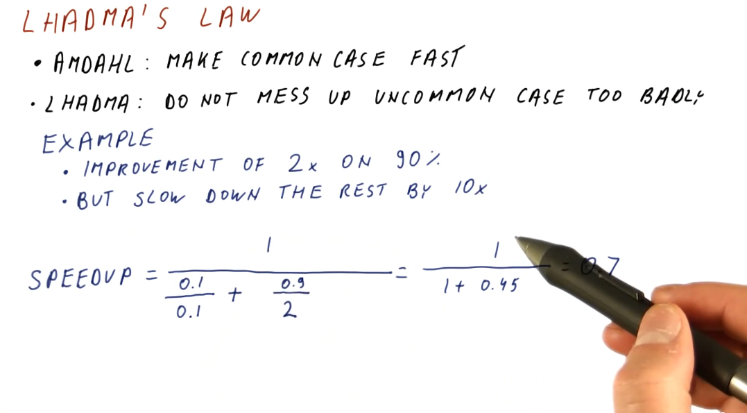
Lhadma's Law

This law is jokingly used to express the opposite of Amdahl's Law. While Amdahl's Law says to optimize for the common case, Lhadma's warns us that we should avoid attempting to optimize too much at the expense of other parts of our performance. An example is provided below.

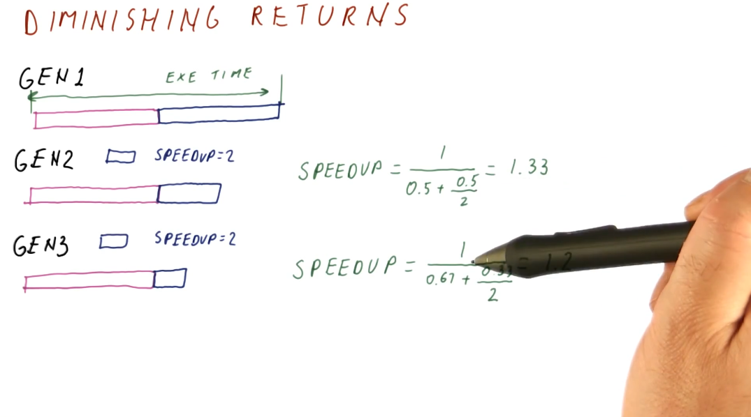
Diminishing returns

This concept covers the idea that as computer architects, we need to continuously review what needs to be enhanced within a system instead of continuously enhancing the same portion of a system. This concept stems from Amdahl's Law, as it describes that, eventually, the enhanced portion of a system will become smaller as we apply enhancements across generations. We will achieve a diminished speedup if we continue to enhance the same portion of the system. We need to continually reassess what is the common case when conducting our enhancements. Below is a high level representation of this idea.

References

1. http://www.tpc.org/tpch/
2. https://www.eembc.org/
3. https://www.spec.org/benchmarks.html
4. Lesson 2 Notes

Pipelining

This lesson reviews pipelining to set the stage for more advanced topics.

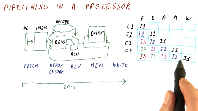
Pipelining in a processor

This section covers basic pipelining in a processor. Most processors are much more complex than the example provided here, however, this is used to review content for students.

In a traditional processor pipeline, we have are series of stages. The following listing of stages is not all stages, but it encompasses the important ones:

• fetch
• read
• decode
• execute
• memory access
• write

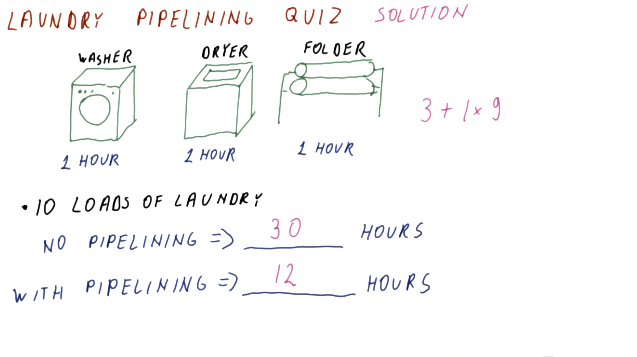
So how does pipelining apply to these stages? Instead of fetching, decoding, and executing one instruction at a time, while one instruction is being decoded, another instruction can be fetched from instruction memory. Then, when one instruction is being executed, we can be decoding the instruction behind it. So, while the latency may not change, the throughput of instructions through the pipeline increases. Below is a high level representation of this concept:

Below is an example of calculating the latency of process with and without a pipeline.

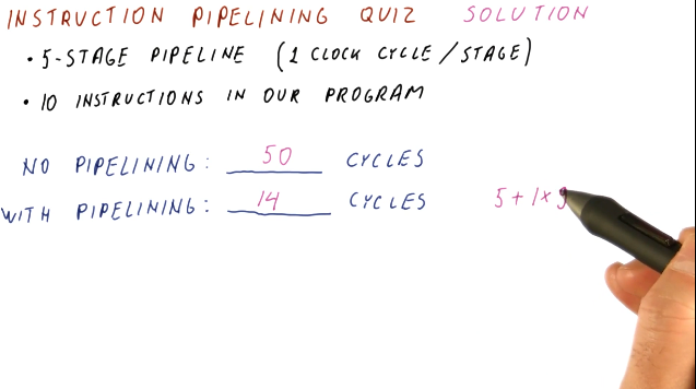
Below is a similar example as the one above, however, this one applies to instructions and cycles.

Pipeline cycles per instruction

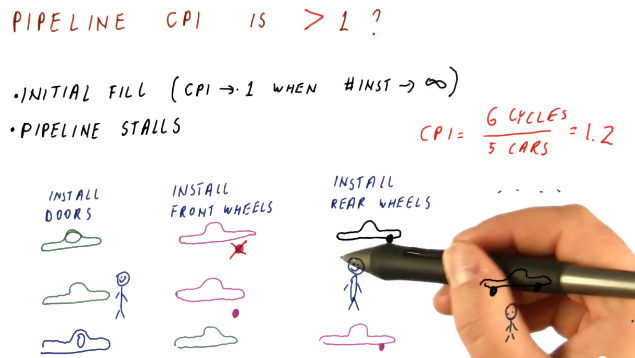
Throughout these notes we've been assuming one cycle per instruction, or a CPI of 1, when our pipeline is full. In the real-world, however, we'll have billions of instructions to execute - will our CPI always be 1? Here are some reasons why our CPI might not be 1:

• initial fill - when the pipeline initially fills up, our CPI will not be equal to 1. Regardless, as our instruction number reaches infinity, CPI will begin to approach 1.
• pipeline stalls - there exists the possibility that a fault occurs in the pipeline and an instruction stalls, causing it to have to remain at that stage for a cycle.

Below is a high-level representation of how a CPI can be greater than 1.

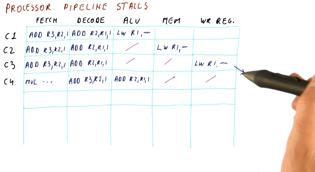
Processor pipeline stalls

A processor pipeline stall usually occurs when some instructions depend upon the outcome of previous instructions that conduct a read/write. In the example below, the program loads a value into a register, increments the register, and then stores that value into a different register. The load operation must occur before the increment and load instruction, otherwise the increment instruction will be incrementing an incorrect value. Because of this dependency, a processor pipeline stall occurs, and a bubble in the pipeline is created. The increment instruction must wait two cycles until the memory is read and written into the register that is to be incremented.

This phenomenon causes our CPI to be greater than 1.

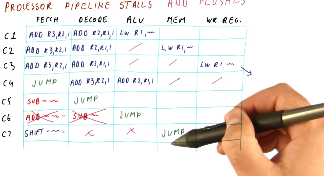
Processor pipeline stalls and flushes

A processor pipeline flush occurs when the processor pipeline fetches and decodes instructions that aren't actually supposed to be executed, so they're removed from the pipeline and replaced with bubbles. Below is an example demonstrating what happens when a JMP instruction is introduced into the pipeline. Some instructions behind the JMP are fetched and decoded, however, they are fetched from an incorrect location in memory. After the ALU determines the destination of the JMP, instructions from the JMP destination are fetched and decoded, and the instructions that weren't destined to be executed are flushed from the pipeline.

This is another phenomenon that could cause the CPI to be larger than 1.

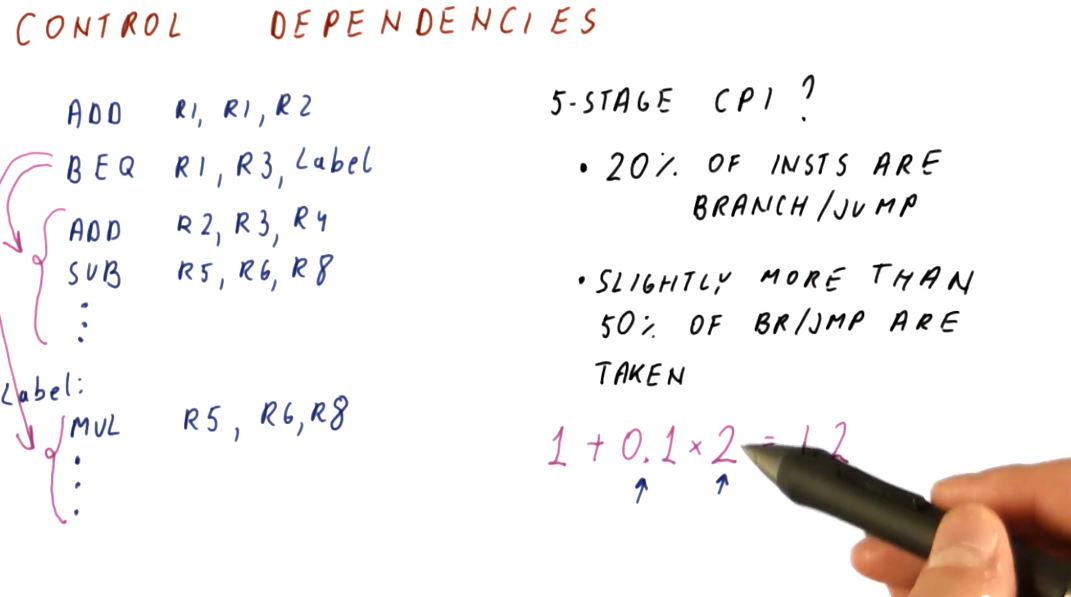
Control dependencies

The problems described in the previous sections that cause these processor pipeline stalls are called control dependencies. The example provided below provides a high-level representation of a control dependency. In the scenario, a branch instruction will jump to some label in code, however, to sections of code depend upon the branch: the code directly after the branch and the code contained at the label.

This example also shows us how to predict the CPI based upon this concept of control dependencies. Given a percentage of instructions are branches, given that a percentages of branches are actually taken, and given that we know that the fetching and decoding of control dependencies causes at least two bubbles in the pipeline, we can calculate the increase in CPI from its normal value of 1.

In later discussions, we will cover a concept called branch prediction that is designed to mitigate the occurrence of these bubbles within the pipeline by predicting where a branch will land in order to fetch and decode the correct instructions. Control dependencies can cause even more bubbles to form in a pipeline if the pipeline contains more than 5 stages, so these issues definitely need to be mitigated to increase performance and normalize the CPI.

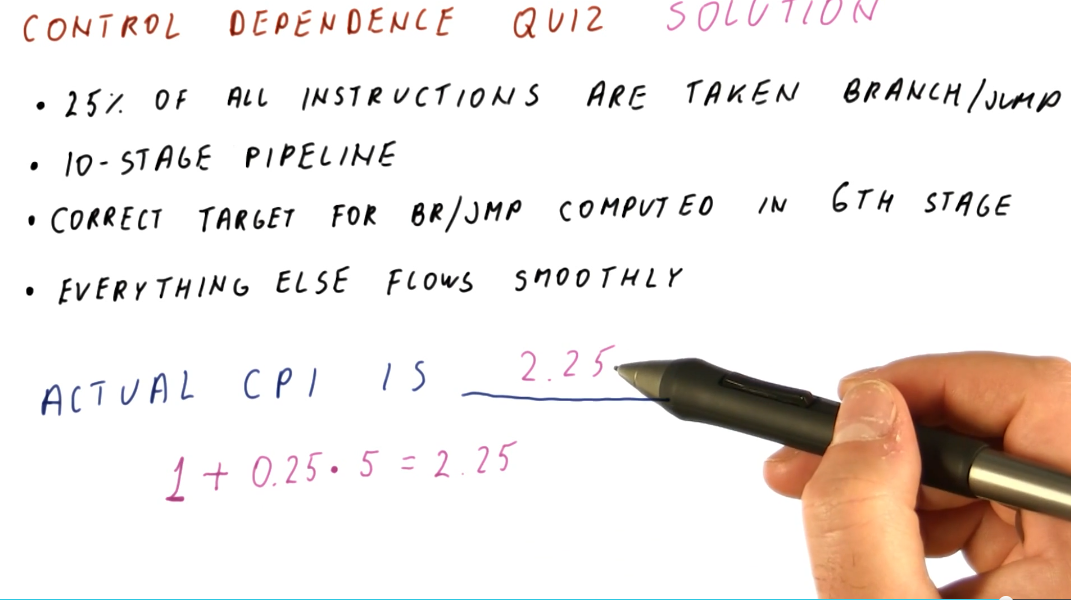
Below is an example question from the lectures that asks us to determine the CPI given a percentage of branches/jumps taken and when the branches/jumps are computed in the pipeline.

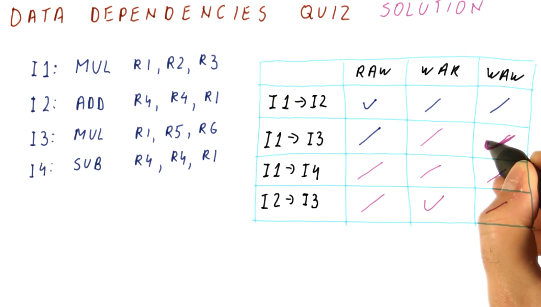
Data dependencies

Briefly described in this section, data dependencies occur when one instruction depends upon the outcome of another instruction. TODO types of dependencies exist:

• read after write (RAW) - type of dependency in which one instruction relies upon the previous instruction writing some data that will be used by the dependent instruction. This type of dependency is also called a flow dependence because the data flows from one instruction to the other. This type of dependency is also called a true dependency because the value being used by the dependent instruction doesn't exist until the previous instruction writes.
• write after write (WAW) - type of dependency in which the order of write operations needs to be preserved. The example provided uses registers, in which a specific value is expected to be within R1 for future instructions. These writes will not be able to to be conducted out of order - they both write to the same location. This type of dependency is also called an output dependency.
• write after read (WAR) - type of dependency in which a previous instruction needs to read some data, but a future instruction intends to write to that data. These instructions can not be interleaved, the previous instruction expects the data to be unchanged upon read. The read will take place before the write, creating the dependency. This type of dependency is also called an anti-dependency because it reversed the RAW dependency.

The WAW and WAR dependencies are called false or named dependencies. Read after read (RAR) is not a dependency.

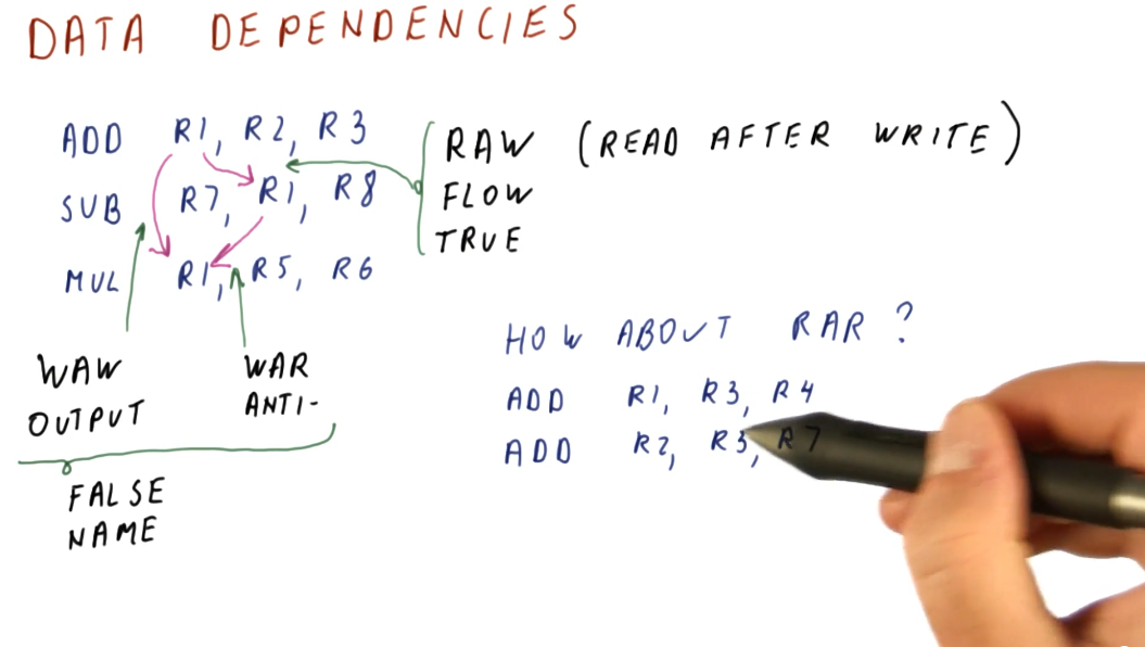
Below is an example from the lectures inspecting a series of instructions to determine what data dependencies exist.

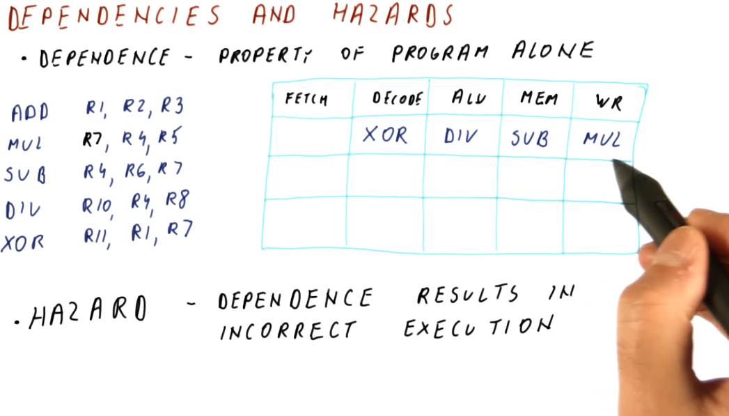
Data dependencies and hazards

A hazard is when a dependence results in incorrect execution of an instruction. In the example provided below, there are three instructions that have dependencies but their dependencies will not result in incorrect values being used for execution.

The DIV instruction, however, will be using a stale value for R4 when it executes and writes to R10 because, when the DIV instruction reaches the decode stage of the pipeline, the SUB instruction has not yet written its value to R4.

Hazards can both be a property of the program as well as because of the pipeline. Another example provided in the image below shows that, in this 5 stage pipeline, true dependencies do not create a hazard when 3 or more instructions separate the dependent instructions. This is because, by the time the first instruction in the dependent pair executes and writes, the second dependent instruction is still being fetched.

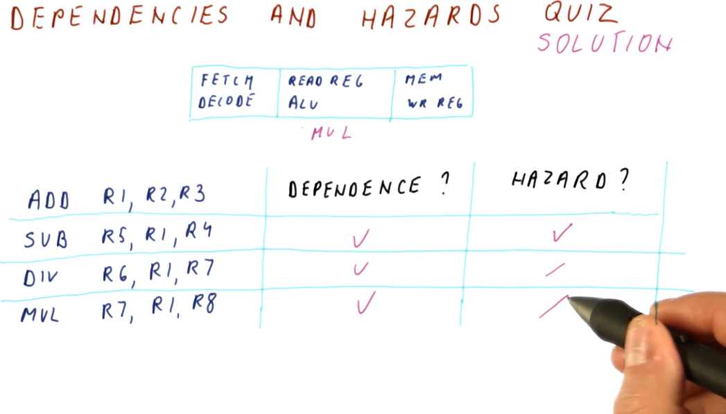
Below is an example problem with a 3 stage pipeline, demonstrating how we can inspect instructions to determine dependencies and hazards.

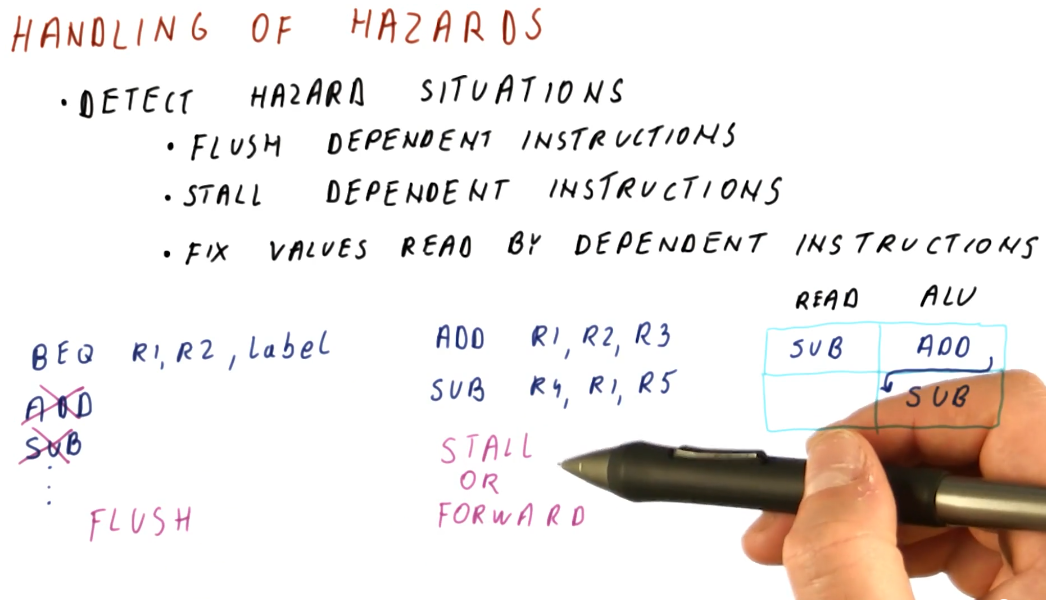
Handling of hazards

We need to introduce mechanisms to handle hazards we detect in order to protect our CPI and performance. We don't care about all dependencies that are introduced, only the ones we know will cause incorrect execution. These are our possible mitigation techniques:

• Flush dependent instructions - used for control dependencies. We don't intend to execute instructions introduced into the pipeline by control dependencies.
• Stall dependent instructions - used for data dependencies in order to prevent instructions from reading invalid values.
• Fix values read by dependent instructions - also used for data dependencies, this introduces the concept of forwarding, providing the a dependent instruction with the value it needs to correctly decode and execute.

Below is a high-level representation of these hazard handling mechanisms.

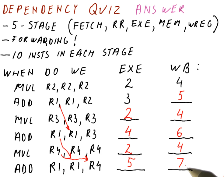
Below is an example problem with a 5 stage pipeline and a series of instructions containing multiple dependencies and hazards that must be avoided. This example demonstrates how we can use the pipeline to determine when it is appropriate to flush, stall, or forward to handle hazards.

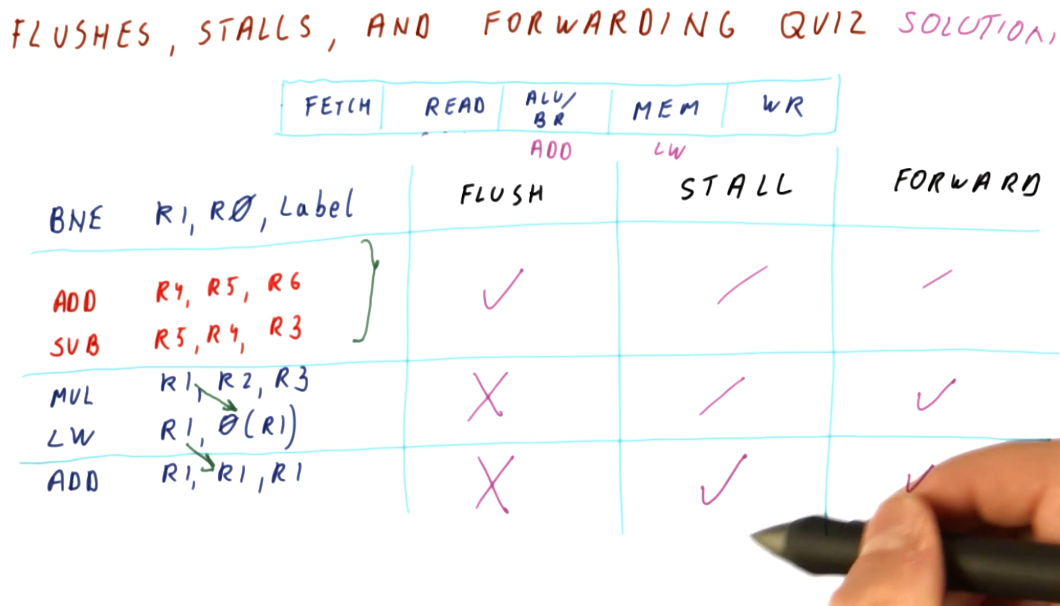
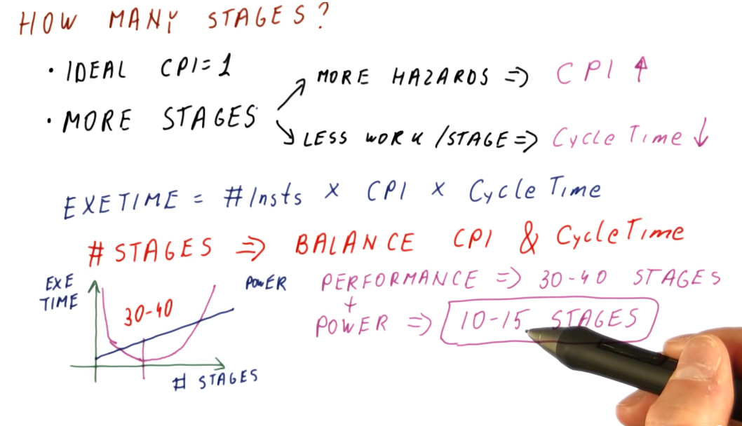
How many stages?

In the pipelines we've reviewed, the ideal CPI is 1. Later in the course, pipelines with a CPI higher than 1 are expected because the pipeline is attempting to execute more than one instruction per cycle. Regardless, each pipeline setup has an ideal CPI that it attempts to achieve.

So what happens if we add more stages? Well, we get more hazards. If a branch is resolved in the third cycle of a pipeline, we only have to flush the two previous instructions that were fetched and decoded. If a branch is resolved in, for example, the tenth cycle of a pipeline, now 9 instructions have to be flushed from the pipeline - kinda wasteful. With more hazards, our CPI also increases.

Inversely, with more stages in our pipeline there's less work being done per stage, decreasing our cycle time - we can execute cycles faster. Remember the Iron Law?

CPU time = #instructions * CPI * cycle_time

If our number of instructions stays the same, but our CPI increases and our cycle time decreases, we achieve a balance even with this longer pipeline. We carefully choose the number of stages in our pipeline to balance the relationship between CPI and cycle time.

Modern processors achieve the most performance with a processor pipeline of 30 - 40 stages as this strikes a perfect balance between cycle time and CPI. This is great, but with an increase in number or processor pipeline stages, we also draw a lot of power because we execute a lot of cycles per second. Thus, a reasonable number of stages for the processor pipeline of modern processors is 10 - 15 stages as this strikes the best balance between performance and power.

Below is a high-level representation of the concepts described above.

References

1. Lesson 3 Notes

Branches

In the previous pipelining lesson, we saw the effects that hazards have on performance. Branches and jumps are common instructions that introduce control dependencies - our only solution can't just be to flush the processor pipeline each time a branch or jump is decoded. This lesson covers techniques used to effectively avoid hazards introduced by control dependencies.

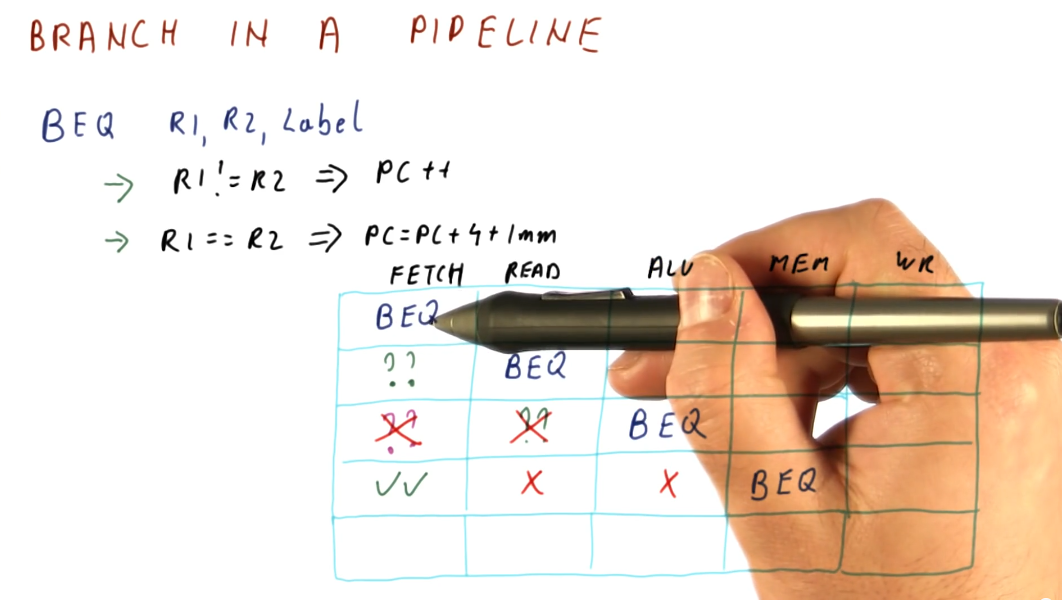
Branch in a pipeline

The example provided below uses a 5 stage processor pipeline to demonstrate the costs of incorrect branch prediction. The example explains how a branch instruction works: is registers R1 and R2 are equal, the immediate value represented by Label will be added to the program counter, PC, and execution will begin at that location in memory. Otherwise, the program counter will be incremented regularly - R1 and R2 are not equal.

In this scenario, a branch instruction enters the pipeline at cycle 1. The branch instruction isn't evaluated until cycle 3 by the ALU. Meanwhile, two instructions are fetched and decoded - these are represented by a ?? because the instructions can be fetched either from memory directly after the branch instruction or the landing location in memory if the branch instruction is taken.

If we predict the outcome of the branch instruction correctly, the instructions that were fetched and decoded will execute immediately after the branch instruction leaves the pipeline - the branch will have taken 1 cycle to complete. If we predicted the outcome of the branch incorrectly and loaded the wrong instructions into the pipeline, these instructions will have to be flushed and the branch will have taken 3 cycles to complete.

References

1. Lesson 4 Notes

Prediction

Branch prediction requirements

What do we need in order to successfully predict whether a branch will be taken or not? What do need in order to determine where the branch is going if it's taken?

The requirements are as follows:

• Branch prediction needs to work using only the knowledge of where we fetch the current instruction from.
  • We need branch prediction to guess the program counter of the next instruction to fetch.
• With branch prediction we must correctly guess:
  • Is this a branch?
  • If it is a branch, is it taken?
  • If it is a taken branch, what is the target program counter?

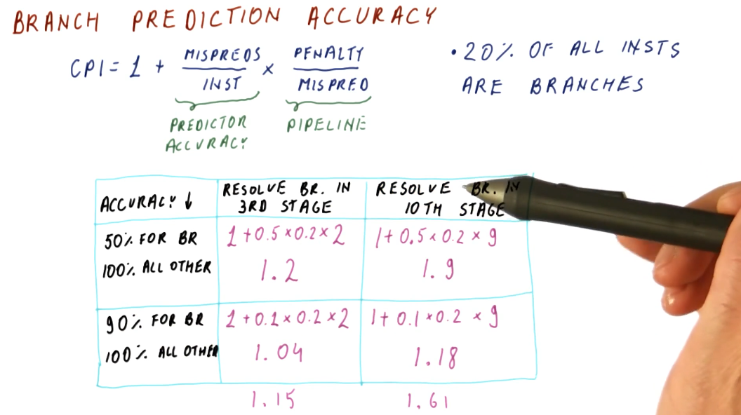
Branch prediction accuracy

The image below demonstrates how we can calculate the theoretical CPI of a processor using branch prediction given its branch prediction accuracy, penalty per missed prediction, and percentage of instructions that constitute branches within a benchmark program. The equation is contains these components:

• base CPI - in the example below, this is 1.
• predictor accuracy - this is the number of mis-predicted branches per instruction.
• penalty incurred - the penalty is dictated by the number of stages in a pipeline and when the branch instruction is evaluated.

A more accurate branch predictor increases our performance, decreasing the number of penalties taken for mis-predicted branches, thus decreasing our CPI. The amount of help a better predictor has changes depending upon how long the processor pipeline is. Longer pipelines benefit more from better branch prediction than shorter ones.

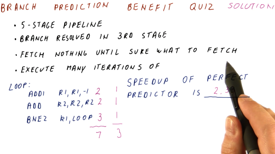
Below is branch prediction example problem. The key to this problem is the fact that no branch prediction is being conducted so, until each instruction is decoded, another instruction will not be fetched, thus creating a bubble within the pipeline. So, non-branch instructions will take 2 cycles to execute and branch instructions will take 3 cycles to execute. Instructions will not be fetched after a branch instruction is decoded because the branch instruction still has to be evaluated prior to fetching from the possible branch destination.

In contrast, each instruction for the perfect branch predictor takes 1 instruction, no bubbles exist within the processor pipeline. This is because the branch predictor knows which instruction will be fetched next before the previous one is decoded - including the branches.

Performance with not-taken prediction

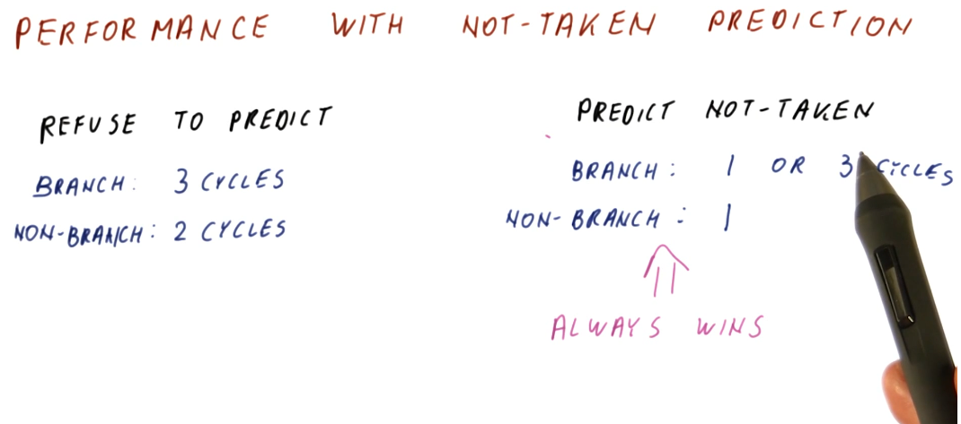
A simple implementation of branch prediction that has an increase in performance over just not predicting branches at all is the prediction that all branches are not taken. If no predictions are made, ever, and instructions are only fetched after previous instructions are decoded, branches will always take 3 cycles in our example 5 stage pipeline and regular instructions will take 2 cycles.

If we always assume the branch is not taken, sometimes we'll be right and the branch will only use 1 cycle, while sometimes we'll be wrong and the branch will use 3 cycles - this is still better than making no predictions at all. In this model, regular instructions only take 1 cycle, as well.

Predict not-taken

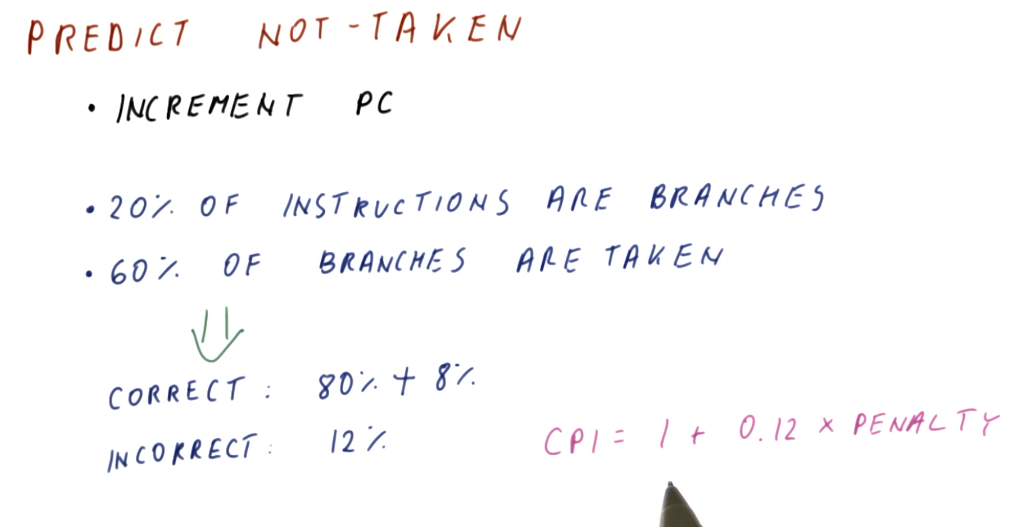
The predict not-taken predictor is the simplest predictor we can have, all it does is increment the program counter. No extra hardware is required to support the predict not-taken predictor - we should always have the ability to increment the program counter.

A rule of thumb in computer architecture is that 20 percent of all instructions are branches. For branches, about 60 percent of all branches are taken. Thus, the predict not-taken predictor is correct 80 percent of the time (because of non-branch instructions), plus another 8 percent of the time (because of branch instructions). Overall, the predict not-taken predictor is incorrect 12 percent of the time.

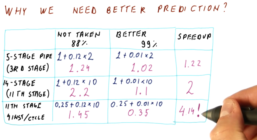
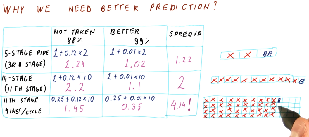
Why do we need better prediction?

The image below provides examples for different types of pipelines, showcasing the differences in performance using a predict not-taken predictor and a branch predictor that is correct 99 percent of the time. As you can see, as the processor pipeline gets longer and more complex, conducting more instructions per cycle, branch prediction becomes really important for performance. The ability to accurately predict branches achieves a speedup of 4 for the case of the 14 stage pipeline with 4 instructions per cycle.

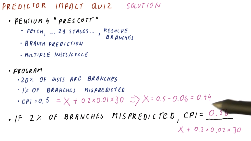
Predictor impact quiz

Below is an example quiz that demonstrates how we can determine the impact of a predictor on the CPI of a processor pipeline. Given some metrics about the Pentium 4 processor, we are given a final CPI but not the theoretically ideal CPI of the pipeline. Using the metrics given, we have to derive the ideal CPI and then calculate the new CPI given a different mis-prediction percentage for our predictor.

Why we need better prediction, part 2

The below image displays how wasteful flushing the processor pipeline is when we fail to accurately predict branches. Depending upon how many stages are within a pipeline, while also accounting for the fact that we could execute multiple instructions per cycle, we see that would fetch and flush anywhere from 2, to 10, to 40 instructions - pretty wasteful.

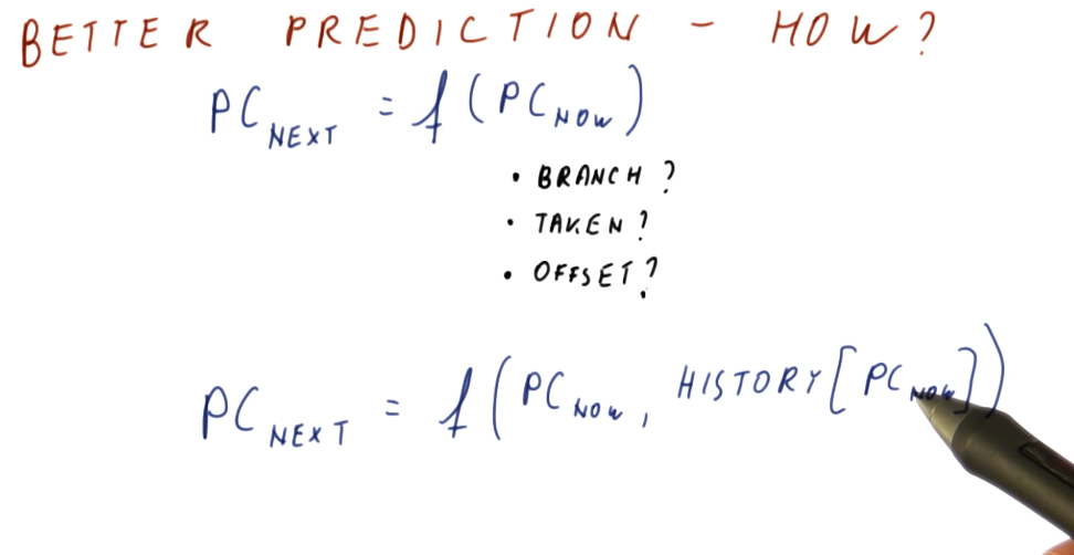
How do we get better prediction?

In a previous section, we discussed the requirements that needed to be met in order to conduct branch prediction. In the image below, the lecture discusses that we don't have the ability to determine if the instruction is a branch, if the instruction is taken, or what the offset of the branch is because we still have yet to fetch the instruction.

What we do know, however, is that, based upon the program counter, we have a historical precedence for what happened at this program counter in the past. We know how the branch at this program counter was behaving in the past - we can use this information because it's pretty common that branches tend to behave the same way each time they are encountered.

We don't know what the current branch instruction to be fetched is going to do, but we can make a prediction based upon its history / the last time it was executed.

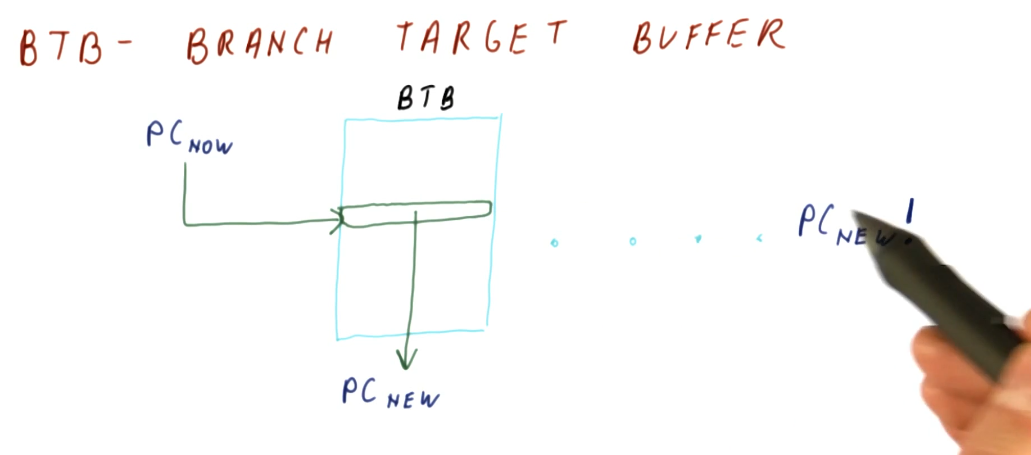
Branch Target Buffer (BTB)

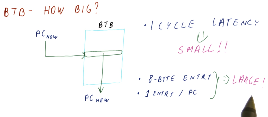
The simplest predictor that uses history is the branch target buffer. So how does it work? The program counter (PC) is used to index into the BTB. Stored at this index is the predicted next program counter. The next program counter is fetched into the pipeline. When the branch is calculated, the real next program counter is determined and compared against the predicted next program counter that was fetched. If they're the same, the BTB predicted the next program counter correctly based upon the historical data saved for the program counter used as an index. If they're not the same, the BTB predicted incorrectly and the next program counter is saved to the BTB using the index program counter.

How big does the BTB need to be to implement the predictor? Well it serves the purpose of predicting the next instruction based upon the current instruction in the program counter. So in order to feasibly predict every next instruction, we need to have an index for every instruction in the program - meaning the BTB needs to be the same size as the program itself! That's not realistic, let's see if we can't find another answer.

Realistic BTB

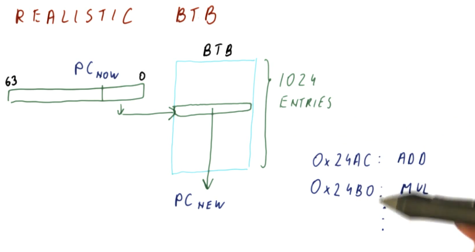
First, we don't need an entry in the BTB for every single instruction in the program - we can have the BTB contain only the instructions that are most likely to be executed next. The BTB will operate somewhat like a cache, using values that are most recently used. An example provided in the lecture is a loop that contains, say, 100 instructions. As the loop executes, the BTB fills with the loop's instructions and the BTB doesn't change for the duration of the loop.

So how do we avoid program counter index collisions in the BTB? We use a mapping function that's simple enough to execute within one cycle. In the example provided, if the BTB contains 1024 entries, we use the last 10 bits of our 64 bit program counters as indices. Why are we using the LSB of our program counters? Because as a program increments, these values are what changes when each instruction is executed.

BTB Quiz

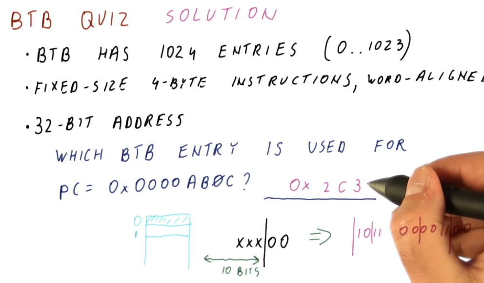
In the quiz below, we would think that we would just use the last 10 bits of the program counter, however, because our architecture enforces 4 bytes instructions that are word-aligned, each entry in the BTB needs to be even and also divisible by 4. So, in a BTB of 1024 entries, we would only be using 256 of the values - that's a lot of wasted entries.

Our solution is to ignore the last 2 bits of the program counter and use the 10 bits to the left of these ignored bits - these bits are the ones that are most likely to change. Using this indexing function, a program counter of 0x0000ab0c will be contained at BTB index 0x2c3.

Direction Predictor

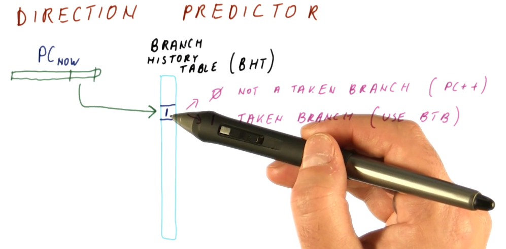
We further simplify our branch predictor by adding another abstraction, the branch history table. This table contains a 1 or 0 for each different program counter that indexes into it - we calculate indices just like we did with the BTB (using the LSBits of a program counter that are most likely to be unique).

The 0 represents that the branch is not taken. The program counter is incremented and we begin fetching instructions from that location. No changes are made to the BTB because no branch was taken.

The 1 represents that the branch is taken. The BTB is referenced to determine the next program counter based upon the current one being inspected, and we begin to fetch instructions from that new location.

If the prediction made is incorrect, the branch history table is updated with the correct value at the index - 0 or 1. If a not taken prediction was made and this prediction ended up being incorrect, we update the BTB with the next program counter that is the destination of the branch.

Because the branch history table is only 1 bit for each index, we can have way more entries for unique program counters. This way, we can use the BTB only for branches and not just regular instructions.

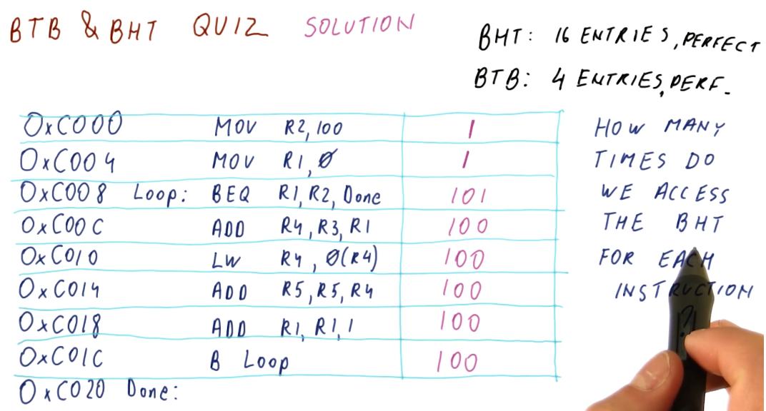
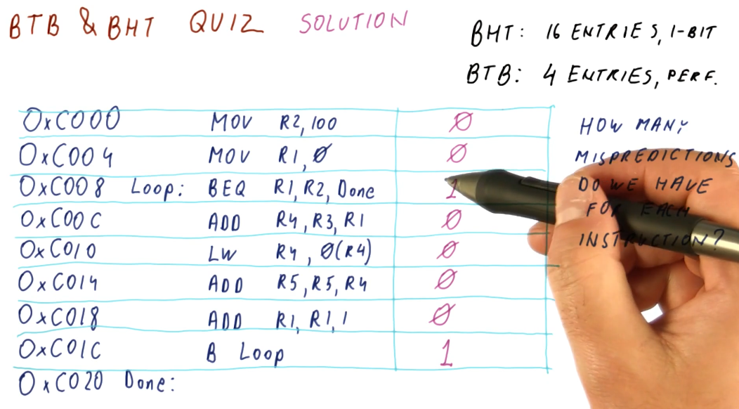
BTB & BHT Quiz

The below quiz excerpt demonstrates that the BHT needs to be accessed for each instruction.

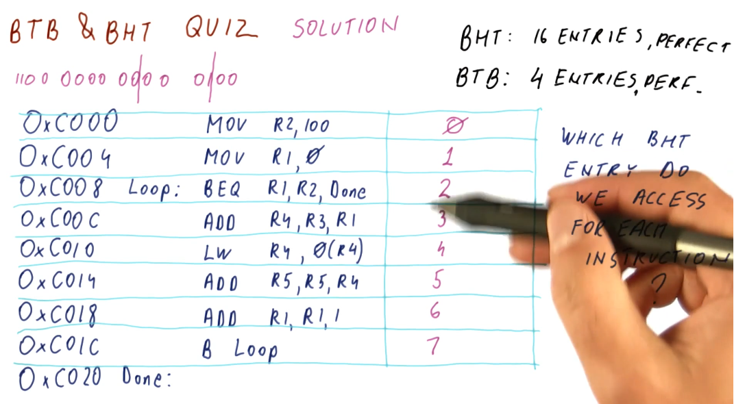
BTB & BHT Quiz 2

The below quiz excerpt demonstrates how the BHT is indexed using the program counter.

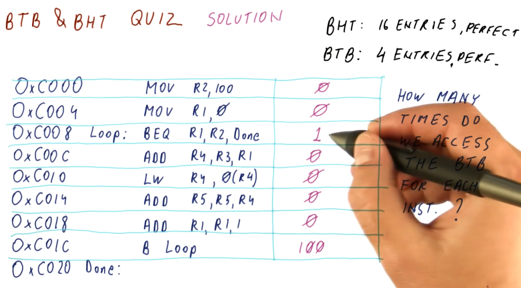
BTB & BHT Quiz 3

The below quiz excerpt demonstrates the conditions required to access the BTB.

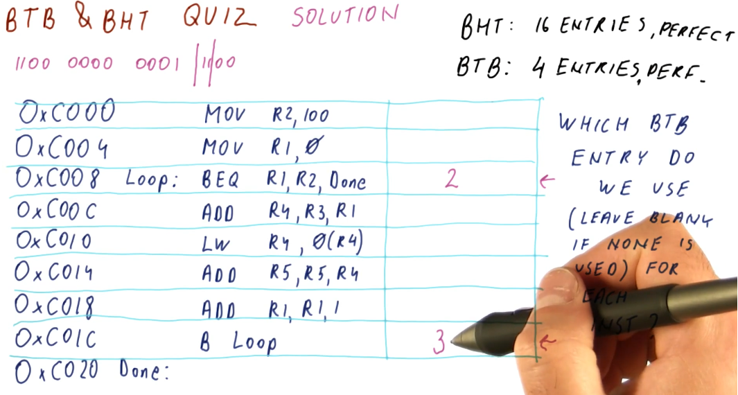
BTB & BHT Quiz 4

The below quiz excerpt demonstrates how the BTB is indexed using the program counter.

BTB & BHT Quiz 5

The below quiz excerpt demonstrates how we can calculate the number of mis-predictions for each instruction using an imperfect BHT.

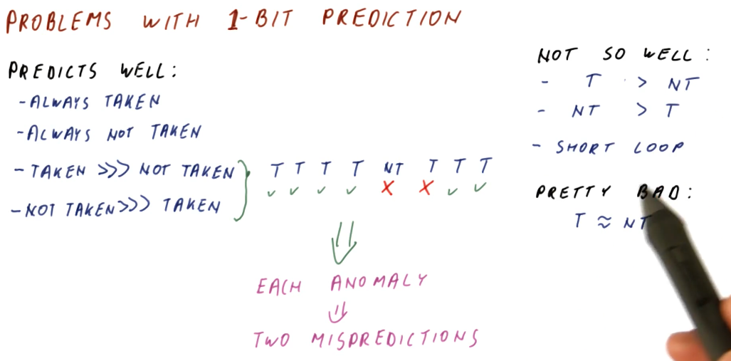
Problems with 1 bit prediction

So what's wrong with the 1 bit predictor? Why does its performance not satisfy the needs of computer architecture designers, creating the need to research pattern predictors?

The 1 bit predictor predicts these things well:

• Branches that are always taken
• Branches that are always not taken
• Branches that are taken A LOT more often than not taken
• Branches that are not taken A LOT more often than taken

The example below demonstrates how, when a 1 bit predictor encounters an anomaly in predictions for a particular branch, this can incur two mis-predictions.

The 1 bit predictor does not perform well when:

• Branches are taken more often than not, but not by much
• Branches are not taken more often than not, but not by much
• Encountering short loops

The 1 bit predictor will be bad when:

• Branches taken and not taken are about the same in number

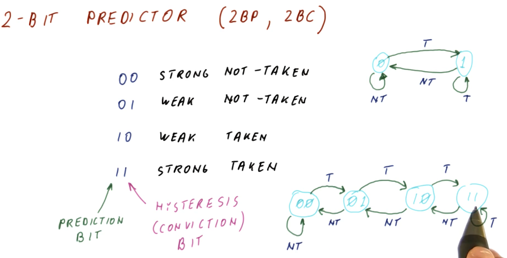
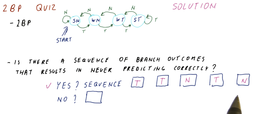
2 Bit Predictor

A 2 bit predictor or 2 bit counter (2BP or 2BC) just adds another bit to the BHT to implement a state machine. The first bit in the 2BP is the prediction bit, and the second bit is called the hysteresis or conviction bit. These are the states of the 2BP:

• 00 - strong not-taken state
• 01 - weak not-taken state
• 10 - weak taken state
• 11 - strong taken state

You can probably see where this is going. We start out in the strong not-taken state for a program counter. When we mis-predict that a branch is not-taken, we increment the hysteresis bit and transition to the weak not-taken state. We still don't take the branch until we are proven incorrectly again. A mis-prediction at this point will transition us to the weak taken state.

So unlike the 1 bit predictor, our affinity to take or not take a branch doesn't flip as easily. This solves the problem we had earlier where, if we encountered an anomaly for a branch that is usually taken or not taken, we won't incur a penalty of two mis-predictions.

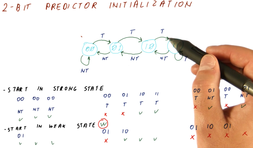
2 Bit Predictor initialization

The below excerpt from the lectures demonstrates that it's a good idea to initialize the 2 bit predictor in a weak state, doesn't matter if it's taken or not taken. This is because, at program start, we don't know the history of the branches, yet, so starting in the weak state only incurs 1 mis-prediction penalty while starting in a strong state incurs 2.

On the flip-side, if a branch flip-flops and we start in the weak state, we will incur a mis-prediction penalty every single time we encounter the branch. This isn't common behavior (fortunately).

The evidence provided above would give you the idea that we should always init the 2 bit predictor in the weak state, but for the sake of practicality, it really doesn't matter and most 2 bit predictors are initialized at 00.

2 Bit Predictor Quiz

The below quiz excerpt from the lectures demonstrates how there is a worst-case scenario for the 2 bit predictor, showcasing a series of branches that will cause the predictor to mis-predict every branch.

The moral of the story is, every predictor will have a worst-case scenario. A good predictor will make it difficult to find or generate this worst-case sequence of branches.

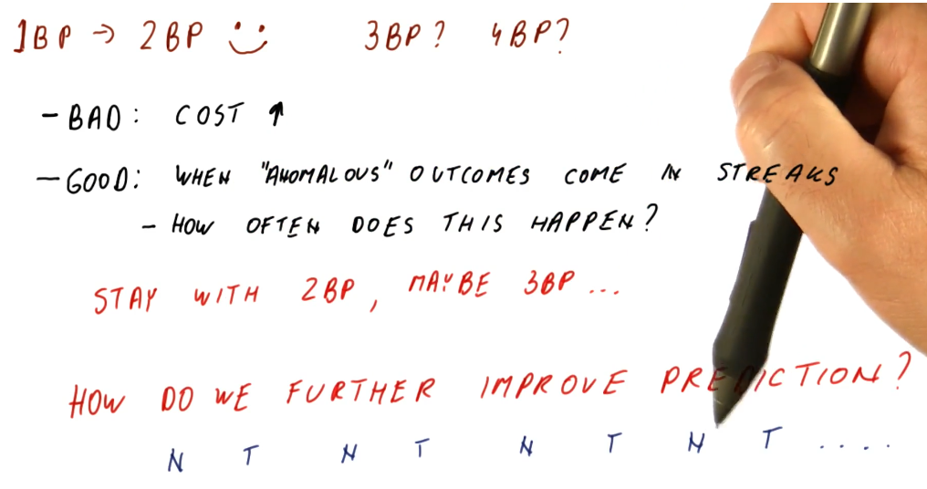
1 bits, 2 bits... what else?

So we've seen that the 2 bit predictor is better than the 1 bit predictor at handling anomalous outcomes. Does this get better if we add 3 bits to the predictor? Well, maybe. Another bit will just increase the number of states, making it more difficult to transition to another prediction - this is useful if the anomalous behavior comes in streaks. This behavior is not common, however , in programs. Adding another bit imposes more cost, as it requires more space to store the information per program counter.

A 2 bit predictor meets the needs we identified earlier of handling anomalous behavior, but what about that one case where the branch outcome kept flip-flopping? Since increasing the number of bits to solve this problem doesn't really do anything, what's the next solution?

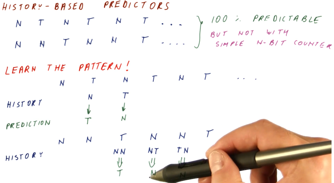
History Based Predictors

History Based Predictors are designed to recognize and learn patterns based upon the history of taken or not taken outcomes of a branch. Below is an example that provides a high-level representation of the concept. The flip-floppy branch outcomes are definitely predictable, just not with simple N-bit counters.

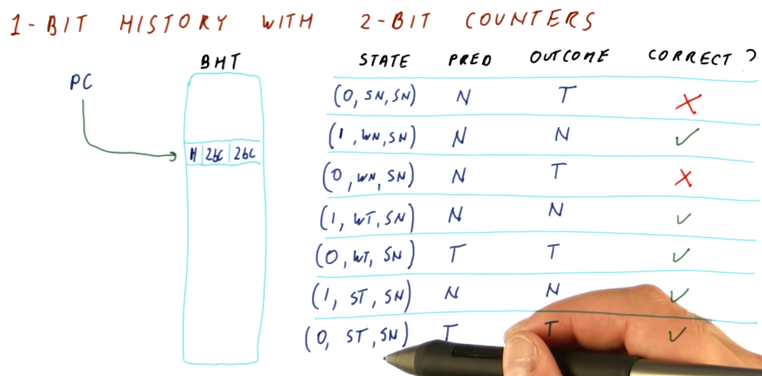
1 Bit History w/ 2BC

Below is an excerpt from the lectures that provides a high-level representation of a BHT with 1 bit for history, and two 2BC's to manage the state for taken and not taken branch outcomes.

What the 1 bit history 2BC BHT provides us is a predictor that is able to learn the pattern of a series of branch outcomes. The 1 bit history bit is used to index into the two 2BC's and, based upon the branch outcome, updates the state of each 2BC.

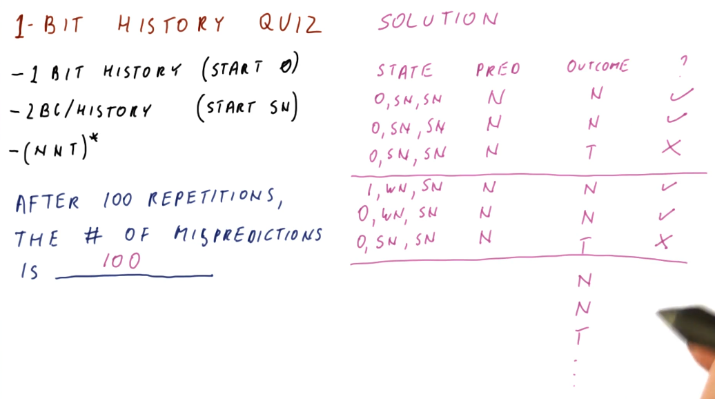
1 Bit History Quiz

Below is an a quiz excerpt from the lectures demonstrating the calculation of the number of mis-predictions for a pattern of branch outcomes following the this pattern: (NNT)*. As we can see from the outcome of the calculations in the quiz, the 1 Bit History with two 2BC's is not a good solution for this pattern.

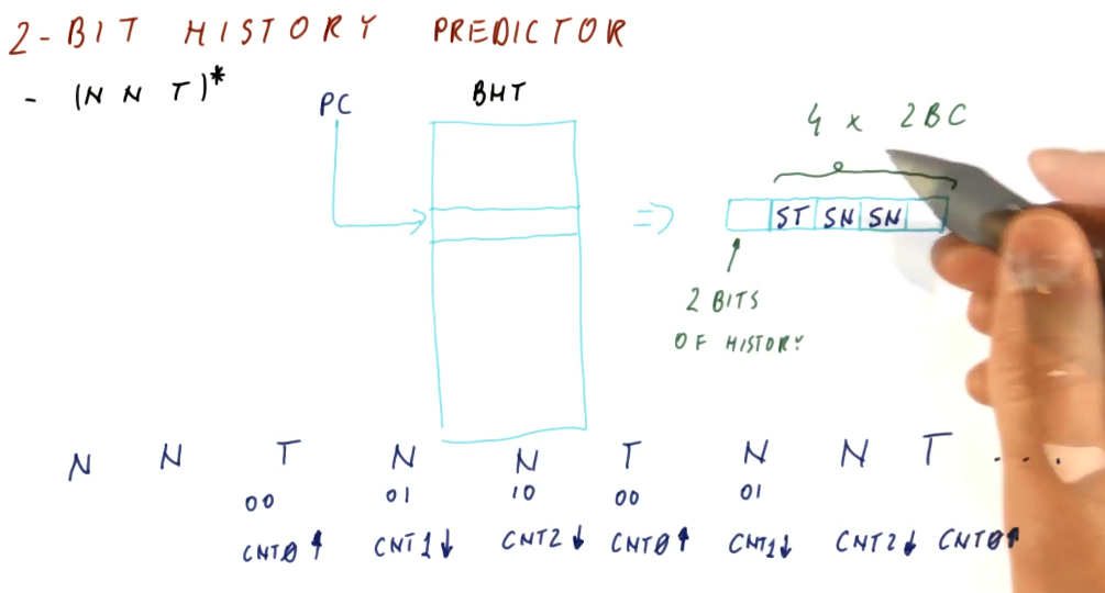
2 Bit History Predictor

The 2 Bit History Predictor works very similar to the 1 Bit History Predictor, now we've just doubled the number of 2BCs. The 2 Bit History bits are used to index into the four 2BCs. The total cost of the predictor is 10 bits per branch. Below is a high-level representation of how a 2 Bit History Predictor can perfectly predict the (NNT)* sequence.

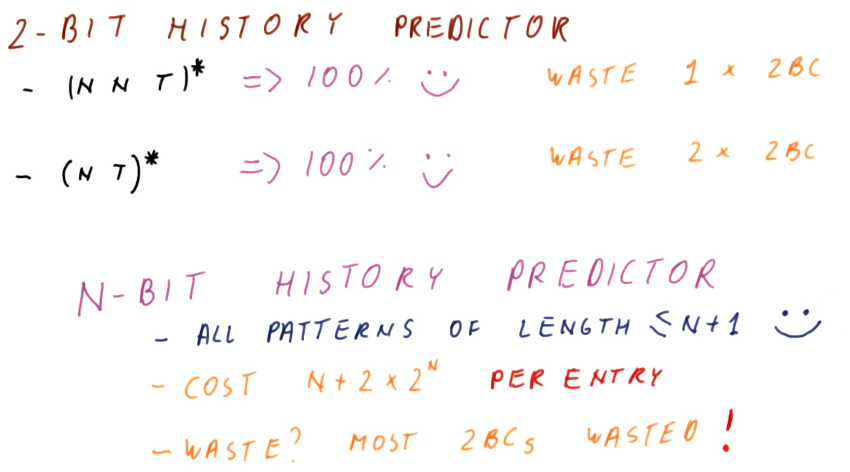
Thinking more about our history predictors, some things become evident. For an N-bit History Predictor:

• We can perfectly predict all patterns of length less than or equal to N+1.
• The cost for an N-bit History Predictor is N + 2 * 2^N per entry
• This is wasteful, most of the 2BCs will go unused.

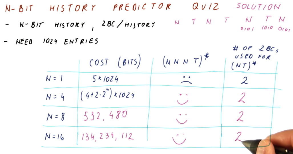
N-bit History Predictor Quiz

The below quiz is an excerpt from the lecture, outlining the cost and waste of different size N-bit History Predictors.

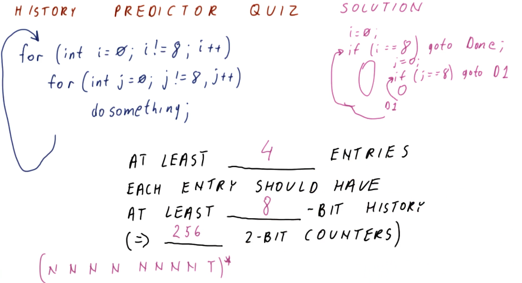
History Predictor Quiz

The below quiz is an excerpt from the lecture, demonstrating how to calculate the number of entries in a history predictor necessary to support a branch outcome pattern generated by these two for loops. As you can see, a lot of 2BCs are wasted just to support an 8 bit history.

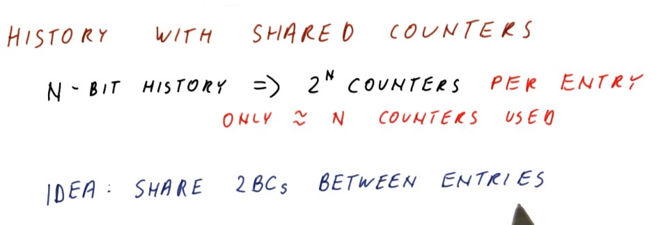
History w/ shared counters

As we discussed earlier, N-bit history predictors use 2^N counter per entry, even when we only use N counters to solve a pattern of N branch outcomes. The idea proposed is to share 2BCs between program counter entries. We only use N counters for N branch outcomes, so with enough counters there's a possibility that we can share without having conflicts.

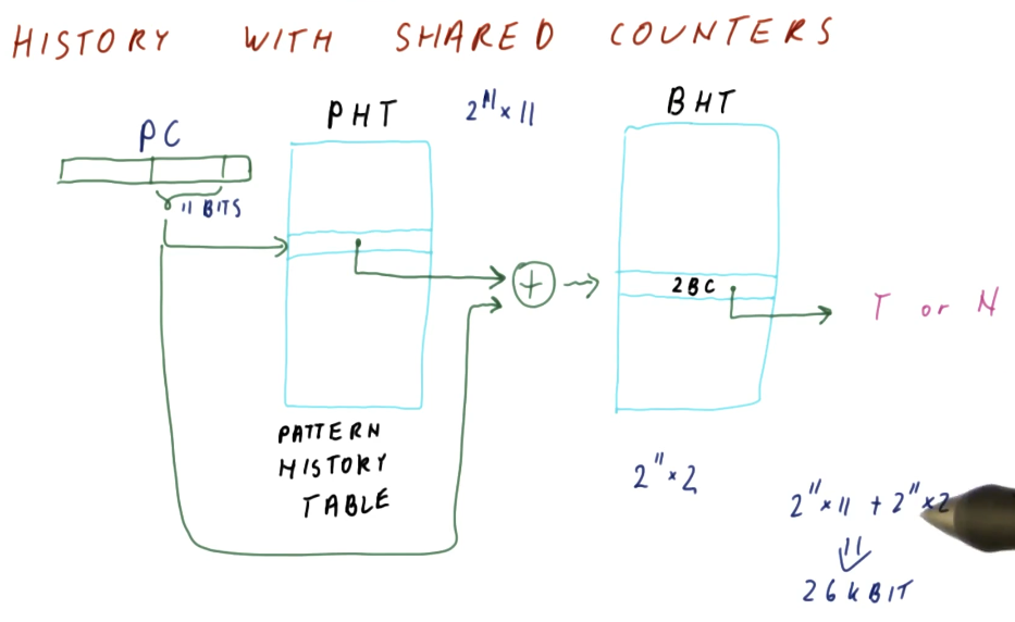
In the excerpt below, we see that designers use the pattern history table abstraction to maintain history pattern history information in a different table , separating it from the BHT. This way, 2BCs can be shared across multiple program counters.

Program counters reference into the PHT in the same way they did with the BTH and BTB, using the least significant bits that are unique. Some translation logic is used to XOR the bits of the program counter and the pattern history information from the PHT to reference the appropriate 2BC for the program counter's pattern.

In this example, the size calculation for these two tables is explained, and the overall cost is much less than the previous implementation of the N-bit history predictor.

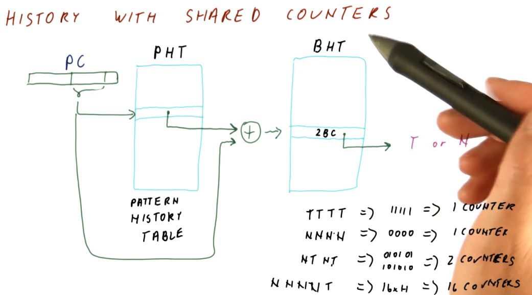
The below excerpt showcases how the BHT is used more efficiently with this design. Patterns that are simple will only end up using 1 2BC, while other patterns that have longer patterns will be able to utilize more counters because less space is taken up by the patterns of other branches. The only cost appended to this design is the creation of the pattern history table. Keep in mind, with the indexing logic shown, it is still possible for branch entries to collide in the BHT.

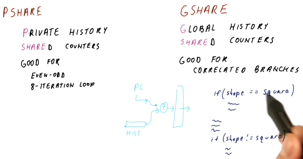
PShare and GShare

The tail end of the history based predictor lesson describes the beginnings of what's known as the PShare predictor. What does PShare stand for? Private history for each branch and Shared counters so that different histories and counters might share the same counter. The PShare predictor is good for flip-floppy branch outcomes and 8-iteration loops.

In contrast, we have GShare with Global history and shared counters. What does global history mean? It means we have single history that is used to predict all branch outcomes. So every history, regardless of program counter, is used to calculate the counter for prediction. The GShare predictor is good for correlated branches.

What's a correlated branch? These are branches whose decisions rely upon what other branches in the program are doing. An example is provided in the excerpt below, showcasing a decision statement where one of two actions will take place depending upon the value of a shape variable. Only one branch will evaluate to try, thus they are correlated branches.

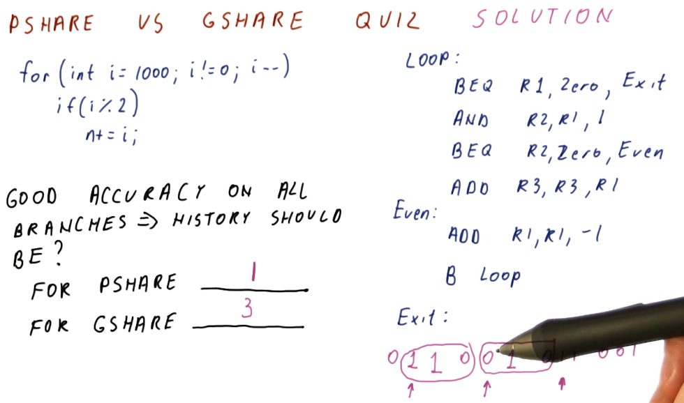
PShare vs GShare Quiz

Below is a quiz excerpt from the class explaining the differences between PShare and GShare. Given some C code, we are provided what the C code would resemble in assembly and then asked to determine how many bits of history would be required to support the branches in the code using both PShare and GShare.

The quiz demonstrates that it would be easy to predict the first and last branches and that they don't require any history support. The first branch will have the outcome of not taken 1000 times, and the last branch will have the outcome of taken 1000 times. The second branch, however, will flip-flop between taken and not taken, as each different integer will evaluate as even or odd. Thus our PShare predictor will need 1 bit of history to support perfect prediction of this branch's outcomes.

In contrast, GShare will require 3 bits of history to support the branches on a global scale and in order to correctly predict the branch outcomes. Again, the first and last branch outcomes are unlikely to change, however, the second branch will flip-flop thus we need 3 bits of history to represent the correlation between these branches. When we see that the first branch was not taken, we'll also see the second branch either being taken or not taken, and if the first branch wasn't taken we know that the third branch is taken.

PShare or GShare

Historically, designers would pick one or the other of these history based predictors. Eventually, designers realized they would need to use both as GShare works well with predicting correlated branches and PShare works better with self similar branches.

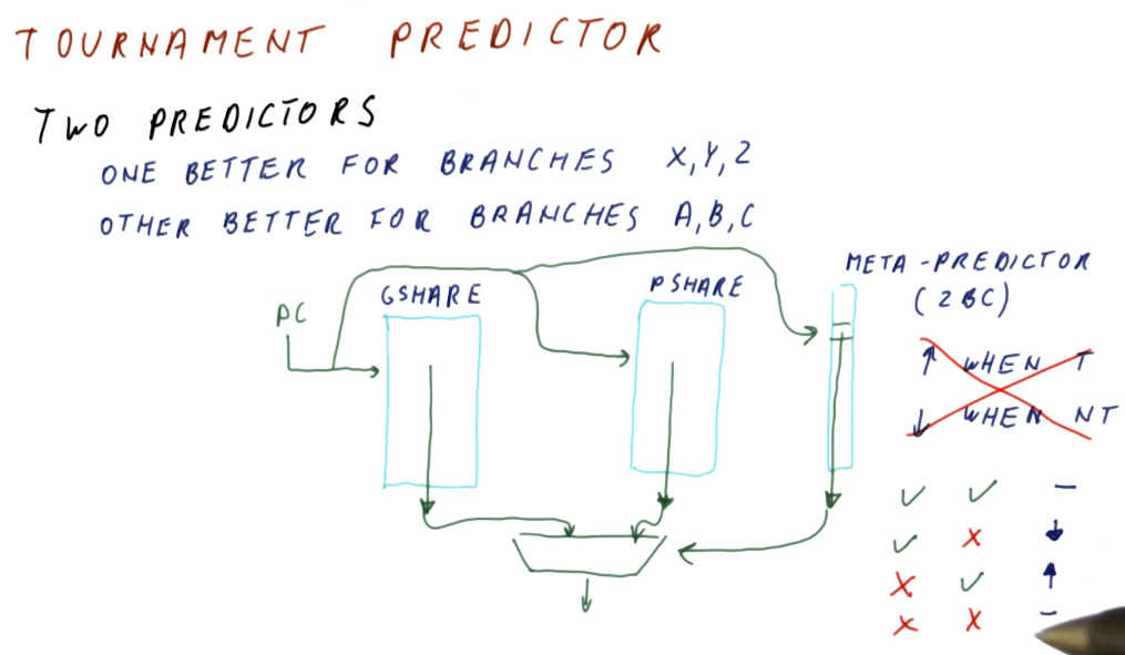
Tournament Predictor

As we discussed in the PShare and GShare section, designers desired to use two predictors to handle different cases of branches - correlated branches and branches that were self similar. But how do we determine which predictor will be used for a program counter (instruction) if we don't know what type of branch it is ahead of time?

The high-level representation below explains how the GShare and PShare predictors are both indexed by the program counter and each predictor provides a predicted branch outcome for that program counter value. At the same time, we use the program counter to index into a meta-predictor table that has a 2BC at each index. We use the meta-predictor to keep track of which shared predictor gives us the correct answer for the program counter the most often.

Return Address Stack (RAS)

So far we've seen branch prediction done for branch and jump instructions, but what about function ret instructions? Functions are designed to be called anywhere, so their ret address will not always be the same location in code. This makes them tougher to predict using our current methods of branch prediction - how do we prevent from fetching instructions from the wrong location when returning from a function?

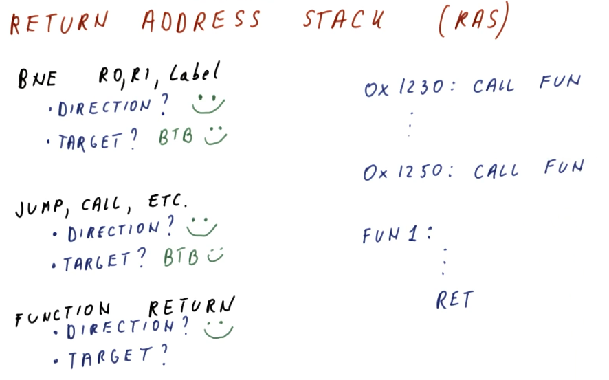
The return address stack is a separate predictor used specifically for predicting returns. It operates similar to the process stack in that it pushes and pops return address for function calls onto the stack. The primary difference between a process stack and the RAS is that the RAS is a very small hardware structure designed to make a prediction very quickly.

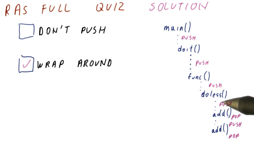
So what happens when the RAS is full and we continue to call into more functions? We have two options:

• Don't push any more return pointers into the RAS
• Wrap around and overwrite RAS entries

So, is it better to wrap around and overwrite RAS entries? The results of a quiz from the class provides the justification for why it's better to wrap around and overwrite RAS entries. In the provided justification below, we demonstrate with a high-level diagram that if we don't push new entries into the RAS when it's full, all we're doing is saving ourselves from mis-predicting older functions calls for functions that aren't getting called often.

In contrast, if we wrap around the entries in the RAS, we're more effectively using the entires we have in the RAS to correctly predict immediate function call returns that are more likely to happen more often.

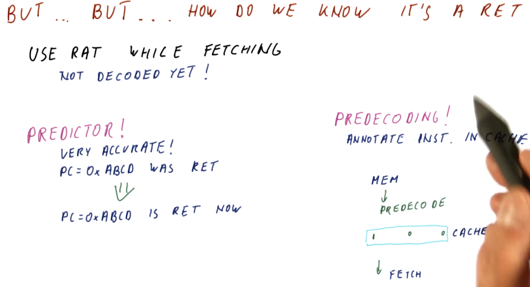
So how do we know the instruction is a ret?

Right, we can't push and pop values to/from the RAS without knowing if the instruction is actually a ret, and we only learn what the instruction is if we fetch and decode. Two methods exist:

• We can use a predictor to determine if the program counter contains a ret. Once the program counter is seen, we now know this program counter contains an instruction that is a ret and we can then push the value onto the RAS.
• We can use pre-decoding!
  • The processor contains a cache that stores instructions that have been fetched from memory. The processor fetches instructions from the cache unless the processor incurs a cache miss - then the process will access memory to acquire the next instruction.
  • Pre-decoding is a process in which we access memory to acquire the next instruction, and as we acquire the next instruction we decode a little bit of it to determine if it's a ret instruction. If it is, we store this information with the instruction in the cache.

Predication

Summary

This lesson covers more topics in relation to control dependencies and the hazards they pose. We covered a bunch of different branch predictors in lesson 4 and we noticed that some branches are really difficult to predict, even when we use really sophisticated branch predictors.

This lesson showcases how the compiler can help us to completely avoid hard to predict branches.

Predication explained

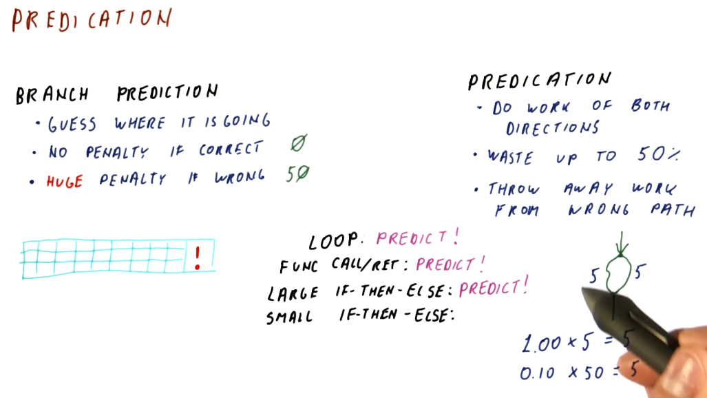
Like we covered in the previous lesson, with branch prediction we attempt to guess the landing location of the branch and we begin fetching instructions from that instruction sequence into the pipeline. If we are correct in our guess, we incur no penalty. An incorrect guess incurs a penalty and, depending upon how long our pipeline is, this penalty can be huge.

Contrast this with predication. In predication, we fetch instructions from the instruction sequences of both possible landing locations for a branch. With this technique, even if we guess correctly or incorrectly, we still have to toss out 50% of the instructions that have been fetched into the processor pipeline. We don't incur a penalty anymore, however, because we realistically aren't making a guess, we're just saying yes to both outcomes of a branch instruction.

So if we're always incurring a penalty with predication, in what context is it better than branch prediction? Here is a breakdown of the examples showcased in the lecture:

• Loops - best application is a branch predictor. Loops are easier to predict as the number of iterations increases. With predication, we would be continuously fetching instructions from the instruction sequence after the loop, wasting a lot of effort as those instructions will continuously flushed from the pipeline - the branch that goes back into the loop will be taken almost always.
• Function calls/ret - best application is a branch predictor. The function will always return, taking the branch instruction. No reason to fetch instructions from the instruction sequence after a ret.
• Large decision statements (if-then-else) - best application is a branch predictor, dependent upon the size of the instruction sequence that comprises the decision statement and the length of the processor pipeline. If two directions in a decision statement were both 100 instructions long and the processor pipeline was 50 stages long, if we mis-predict we only incur a penalty of 50 stages. If we predict correctly, we incur no penalty. In contrast, a predicator will always incur the penalty of 100 because we load instructions from both possible instruction sequences following the branch instruction.
• Small decision statements (if-then-else) - the best application is predication. If two instruction sequence outcomes for a branch are both 5 instructions long, we will always incur a 5 instruction penalty with predication. If we use branch prediction and the processor pipeline is 50 stages long, if we make a mis-prediction, we'll have wasted 50 stages. Dependent upon how accurate the branch predictor is, we might be able to match the performance of predication in this use case, however, the more inaccurate the branch predictor the less viable an option it will be for small decision statements.

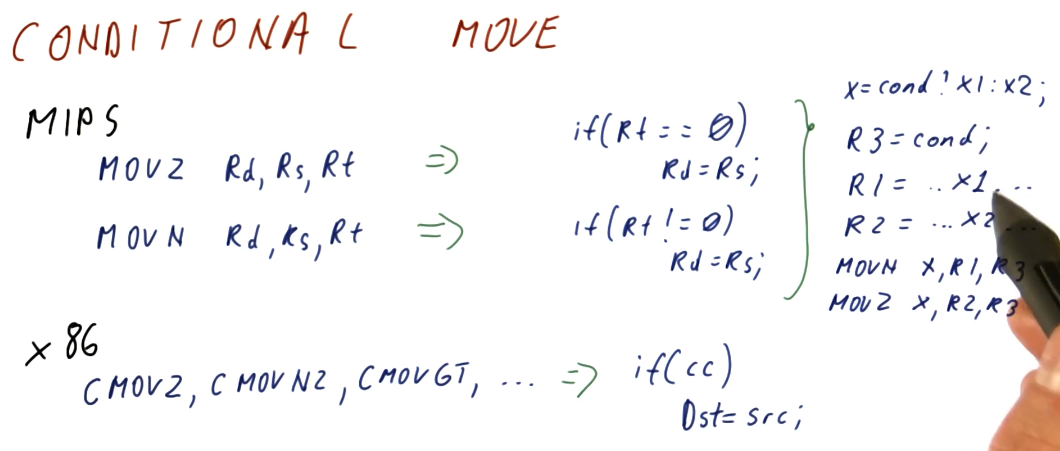
Conditional move

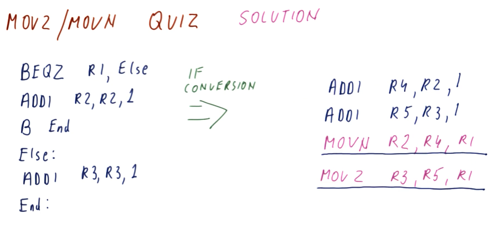
This section discusses the conditional move instructions available in the MIPS and x86 instruction sets. The example below covers MOVZ and MOVN:

• MOVZ - takes two sources and a destination register. If the third operand is equal to 0, the second operand is loaded into the destination register.
• MOVN - takes two sources and a destination register. If the third operand is not equal to 0, the second operand is loaded into the destination register.

Example x86 CMOV instructions are shown below.

MOVZ MOVN quiz

Below is quiz a on how to convert code that originally contains branch instruction into code that uses conditional moves to avoid making predictions. This code models a short decision statement that loads some values into different variables based upon some condition statement.

MOVZ MOVN performance

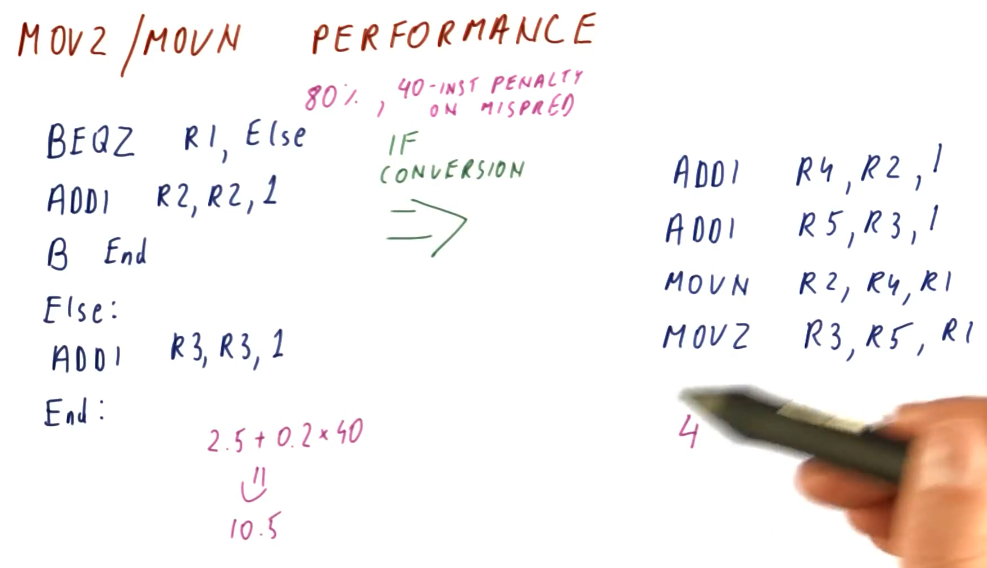
The excerpt from the lectures below showcases a comparison of the performance between traditional branch prediction and the translation we did of the instructions to enable predication. Give a branch predictor that's correct 80% of the time and incurs a 40 instruction penalty if we encounter a mis-prediction, we average the number of instructions that can executed between the two branch instruction sequences, 5 * 0.5 == 2.5, and then we throw in our inaccuracy and penalty: 2.5 + 0.2 * 40 == 10.5.

So, on average, the branch predictor in this example incurs 10.5 instructions worth of work to evaluate and execute this condition statement. In contrast, for predication, all of the instructions are fetched and executed because we've translated the branch into conditional move instructions. We incur 4 instructions worth of work to evaluate and execute this condition statement.

MOVx summary

To summarize predication using MOVx:

• Needs compiler support to translate eligible condition statements using MOVx instructions rather than generating branch instructions
• Removes hard-to-predict branches, increasing performance
• More registers are needed in order to support predication using MOVx
  • Results from both instruction sequences have to be calculated and stored
• More instructions are executed
  • No branch prediction is conducted, both instruction sequences are executed and their results are stored in registers
  • MOVx is used to select the results of the condition statement

So what portions of this summarized list are absolutely necessary to implement predication? Well:

• Compiler support is definitely necessary
• The whole purpose of this is to remove hard-to-predict branches
• We don't need more registers to store our results - we can conduct comparison directly against values in memory
• We don't need to use MOVx to select results

How do we remove the unnecessary portions of the summarization above? We make all of our instructions conditional! With this, we can achieve full predication - but it requires extensive support in the instruction set.

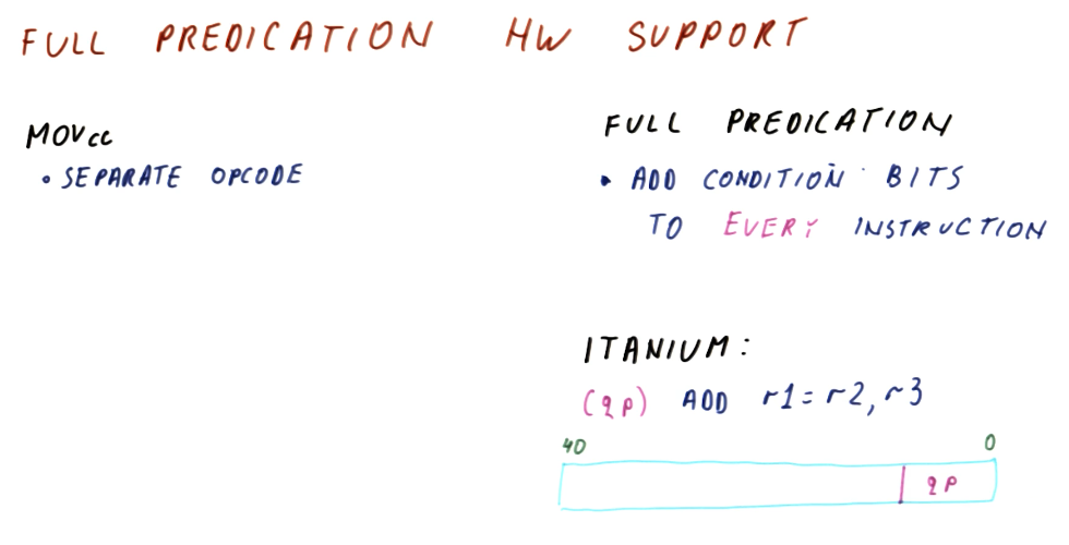
Hardware support for full predication

Usually, we have a separate opcode for conditional move instructions. For full predication, we add condition bits to every instruction. Below is an excerpt from the lectures showcasing the Itanium instruction set's use of qualifying predicates in its instructions to support full predication. Qualifying predicates specify what register will be used to conduct a comparison for a conditional move.

Full predication example

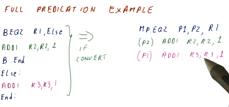
The excerpt below now shows our previous condition statement convert to a set of instructions that uses full predication. The first instruction sets the qualifying predicates, p1 and p2, to 0 or 1 based upon the value of R1 . If R1 is 0, p1 is set and the instruction predicated by p1 will actually store its value into R3 after execution. If R1 is not 0, p2 is set and the instruction predicated by p2 will store its value into R2 after execution.

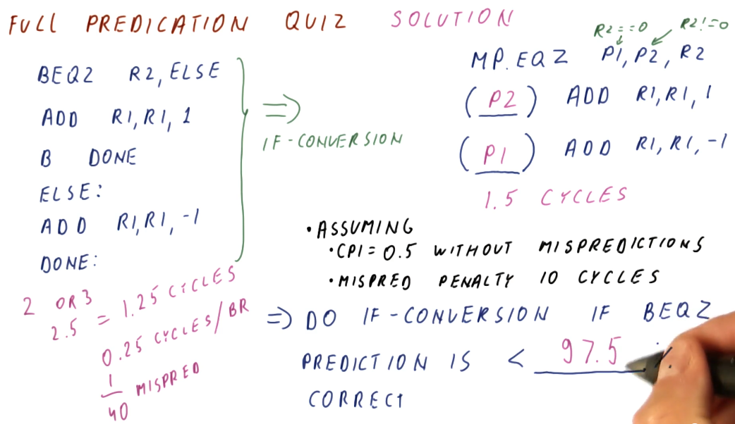
So, in the original code with branch instructions, we have the possibility of executing 2 or 3 instructions based upon our prediction, but we still incur a penalty. In our previous examples using MOVx, we were able to translate the condition statement into a set of 4 instructions. Now, with hardware support for full predication, we are able to translate this condition statement into 3 instructions.

Full predication quiz

Below is a the full predication quiz solution from the lecture, conducting a performance comparison between the original branch version of the condition statement code to the full predication translation.

References

1. Lesson 5 Notes

Instruction Level Parallelism (ILP)

Parallel instruction execution

The below excerpt from the lectures showcases the hazards that can manifest due to data dependencies in parallel processor pipelines. As you can see here multiple instructions are destined to be executed and, if all instructions are able to be executed in parallel, it will take 5 cycles to execute a number of instructions. As the number of instructions approaches infinity, our CPI approaches 0.

This isn't realistic - some instructions will depend upon earlier instructions to write values to registers before the instruction is executed. If this isn't done, we will encounter data hazards wherein the registers we use for our instructions will contain stale values, ultimately causing the program to execute incorrectly.

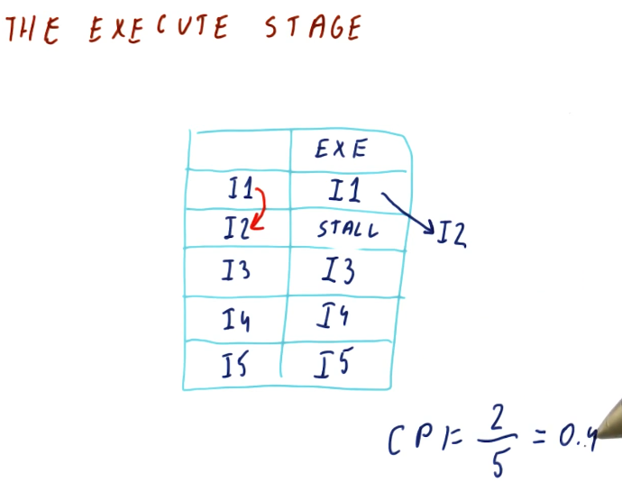
The execute stage

In previous sections of this notebook we discussed forwarding, a technique that can be used to resolve data dependencies and remove hazards. Unfortunately, this technique wont' work for us when we're executing instructions in parallel. The instruction that contains the data dependency will not receive the outcome of the forwarded instruction before it executes because they are executed in parallel.

In order to remove the hazard related to this data dependency, we must stall the instruction until the previous instruction executes. Then, we will forward the result of the executed instruction to the dependent instruction. This will increase our CPI.

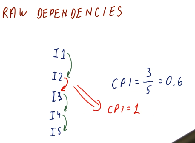
RAW dependencies

The below excerpt from the lectures showcases how we can calculate the CPI for a set of instructions based upon the number of data dependencies that exists between them. As you can see, the more RAW dependencies that exist, the higher our CPI.

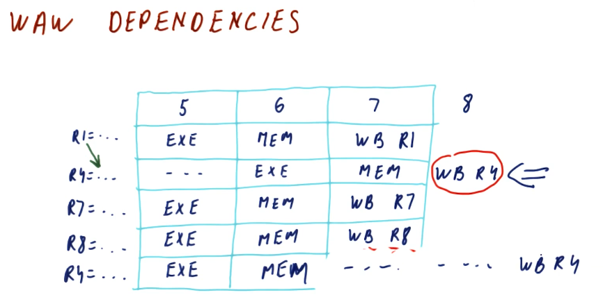
WAW dependencies

The below excerpt from the lectures showcases how a WAW dependency can manifest due to a RAW dependency in previous instructions. The WAW dependency poses a hazard because the previous instruction is stalled due to a RAW dependency. If this goes ignored, the dependent instruction in the WAW dependency will write to a register before the previous write, executing instructions out of order. In order to solve this, the dependent instruction must be stalled twice so that the previous instruction can write.

Dependency quiz

Below is a quiz from the lectures in the class that showcases how multiple RAW and WAW dependencies are handled in the processor pipeline.

False Dependencies

We covered this in previous portions of this notebook, but we'll go over the dependency types once again. We have true dependencies and false or name dependencies. A true dependency is the RAW (read after write) dependency - pretty obvious because this is how the program is actually intended to execute. Both the WAR (write after read) and WAW (write after write) dependencies are false dependencies. In both of these dependencies, we are re-using registers for instructions when we could change the registers being used to eliminate the false dependencies completely.

Duplicating register values

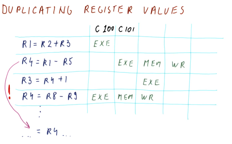
This is a complicated technique in which we save multiple versions of a value for a register that is being written to. In the excerpt below, two different writes occur for the register: R4. This register is used in two different read operations, but what value will be used if the register is written twice?

To remove the hazard posed by this WAW dependency, we store both versions of R4 and then each read operation will utilize the appropriate version based upon the chronological order of the writes. The third instruction in this example will use the outcome of the write in instruction two for its read operation, even though instruction four writes to R4 before instruction two does. A future instruction will use the most previous version of R4 for its read operation, even though the write by instruction two occurs after the write by instruction four.

Essentially, we are keeping track of all possible versions of a register in a parallel pipeline and different read operations that require the value of register will use the value generated by the most recent write operation.

Register renaming

So duplicating and managing register values can get pretty complicated and time consuming. Another technique processors can use to remove hazards created by data dependencies is register renaming.

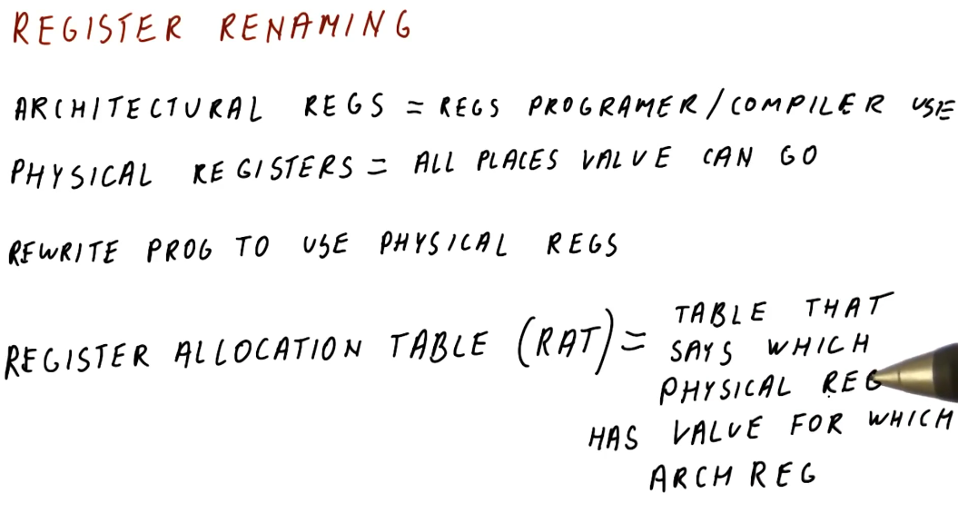
In the below excerpt from the lectures, we define some terms:

• architectural registers - these are register names used by the programmer and the compiler.
• physical registers - these are the physical registers available to the processor to actually store real values.
• register allocation table - this is a table used by the processor to translate architectural register names to physical registers. This table defines which physical register contains the data for a specified architectural register.

The processor rewrites the program it's executing to use the physical registers. Through register renaming, it will have more registers available to store values and avoid hazards presented by data dependencies.

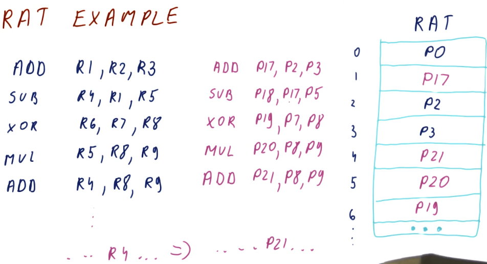
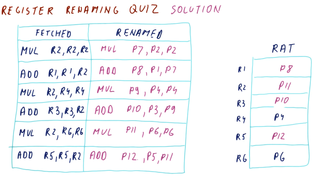
RAT example

The below excerpt from the class showcases how a RAT works. Each time a new value is produced, a different physical register is used to store that value. Values for registers that are being read are acquired from the RAT after it translates the architectural name to the physical register. We call the WAW and WAR dependencies name dependencies because the name is the whole problem. If we rename the register that the value is being written to for each write, the instructions won't overwrite the work of the other instructions if they're executing in parallel.

In this example, we can see that each write increments the physical register number that's being written to. This removes the hazard of a register being overwritten by a later instruction before an earlier instruction can conduct its write. Because the writes are to different physical registers, when an instruction is decoded and needs to read a register, the value it's reading is going to be from the instruction prior, not the most recent write to the register.

Register renaming quiz

Below is a quiz for register renaming from the lectures. Pretty straightforward.

False dependencies after renaming

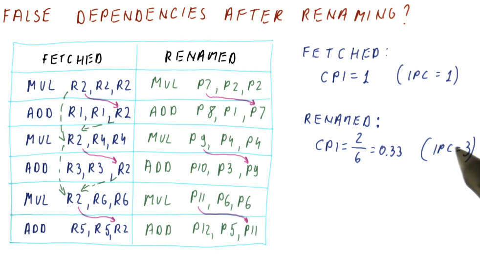
So does renaming actually remove our WAR and WAW dependencies? Yes! In the below excerpt from the lectures we are shown a program that contains a set of dependencies for each instruction. Because each instruction has these dependencies, they must be executed in order, causing us to have a CPI of 1. However, with renaming, we are able to eliminate the WAR and WAW dependencies improving our performance to a CPI of 0.33.

What is ILP?

Instruction level parallelism (ILP) is a property of a program given the fact that it's running on an ideal processor. What's an ideal processor? An ideal processor has these attributes:

• Processor dispatches an entire instruction in 1 cycle.
• Processor can do any number of instructions in the same cycle.
  • The processor has to obey true dependencies when doing this.

So what are the steps to acquire the value of a program's ILP? A program's ILP is equal to the IPC when executing on an ideal processor following the rules stated above. Obviously ideal processors like this always aren't achievable, the ILP for a program will be different on actual real-world processors. ILP gives us a value, however, for the parallel nature of program - defining how many true dependencies exist within the code.

The steps to acquire the ILP of a program are:

1. Rename the registers, as shown previously.
2. "Execute" the code on the ideal processor.

ILP example

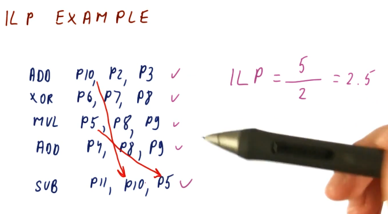
The below excerpt from the lectures showcases how we can compute the ILP for a given set of instructions: ILP == num instructions/cycles. In this example, the professor identifies the true dependencies that exists for the set of instructions and sees that the fifth instruction cannot execute until the writes of instruction one and three are complete. Thus, this program will take 2 cycles on an ideal processor to execute.

A neat trick that is described in the lecture is that we don't even have to conduct register renaming in order to calculate the ILP. All we have to do is identify the true dependencies - the register renaming will take care of the false or name dependencies for us.

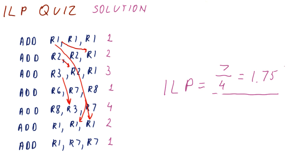
ILP quiz

Below is a quiz from the lectures showcase the technique for calculating ILP described above. We don't conduct register renaming, we just identify the true dependencies to determine on what cycle instructions are eligible to execute. After we determine the minimum number of cycles to resolve the true dependencies, we can find the ILP of the program.

Calculating ILP with structural and control dependencies

When calculating ILP, we don't account for structural dependencies. These dependencies result for architectural issues like not having an adder available for a specific operation, etc. Something outside of the programmer's control, solely relies with the manufacturing of the processor.

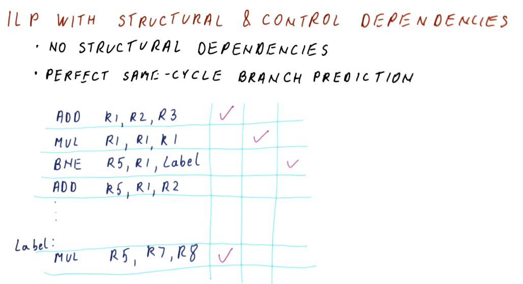
For control dependencies, we essentially ignore them. We assume that we have perfect same-cycle branch prediction. In the example below, we show that a branch instruction has a data dependency on instructions prior to it, however, because we have perfect branch prediction we know that we will jump to the Label. Thus, we fetch the instructions from the Label and execute them, even though our branch has not been executed, yet.

ILP vs IPC

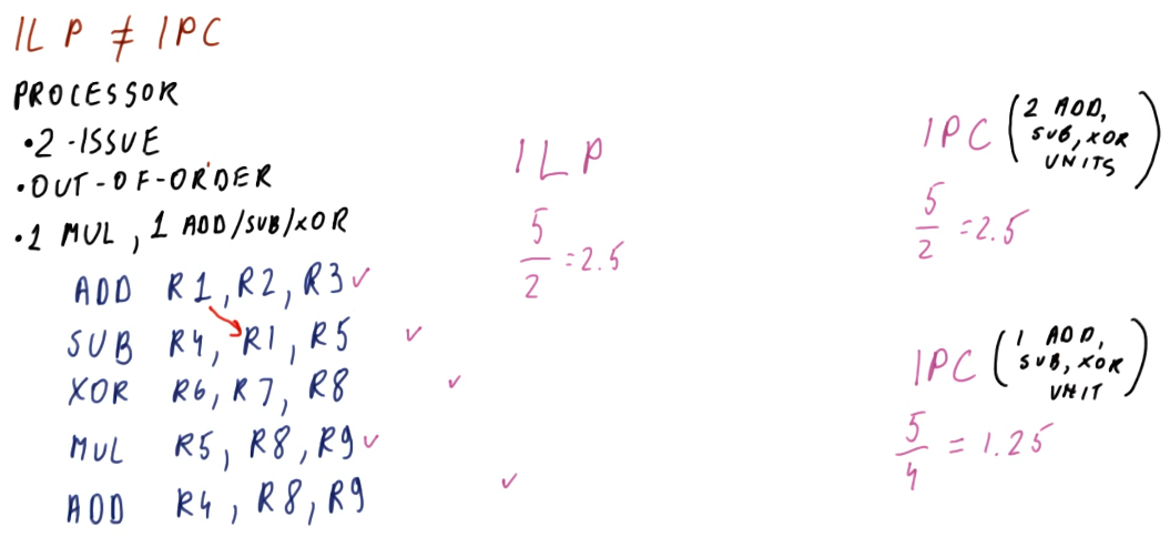
Below is an excerpt from the class conducting a comparison of the calculations for ILP vs IPC on a given example processor. The processor has some limitations such as: 2-issue (2 instructions / cycle), 1 MUL and 1 ADD/SUB/XOR components (structural limitations). With this, we calculate the ILP for the given instructions and then we calculate the IPC twice: once ignoring the structural limitations and once factoring in the structural limitations.

As we can see, the IPC for a processor can only be equal to or less than the ILP. Real processors will have limitations and won't always be able to achieve the ILP of a program.

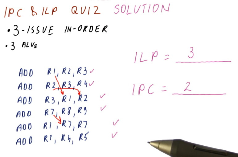
ILP vs IPC quiz

Below is a quiz from the lecture that shows us how to calculate and compare the ILP and IPC of a program for a given test processor. Note, the processor in this example can only dispatch instructions in order, thus degrading our performance in comparison with the out of order processor's we've seen in the past. This limitation causes us to have to stop dispatching instructions when we encounter a dependency.

ILP vs IPC discussion

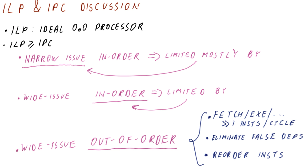
This slide sorta restates what we covered earlier - a summary, essentially. The ILP can only be calculated using the abstract concept of an ideal processor, and it's generally representative of the best performance of a program. The ILP will always be greater than or equal to the IPC, and the IPC is calculated using an actual processor with issue and structural limitations.

The limitations for processors and how they affect IPC breaks down like this:

• If a processor narrowly issues instructions (1 - 2 instructions / cycle), and only executes instructions in order, the processor will mostly be limited by the narrowly issued attribute.
• If a processor widely issues instructions (4 or more instructions / cycle) , and only executes instructions in order, the processor will mostly be limited by the in order attribute.
• The best case is when the processor widely issues instructions but also can execute instructions out of order. To do this, the processor will have to dispatch a lot of instructions per cycle, eliminate false dependencies through register renaming, and reorder instructions so they can be executed out of order.

Instruction Scheduling

This lesson covers how instruction scheduling allows us to execute programs faster by dispatching more than one instruction per cycle while also handling data dependencies.

Improving IPC

As we've seen in previous lectures, there are multiple ways for us to improve IPC:

• Handling control dependencies - if we have good branch prediction we can better handle control dependencies, allowing us to fetch the correct instructions and avoid wasting cycles.
• false data dependencies - when we encounter false or name dependencies (WAR and WAW), we use register renaming to completely eliminate the hazards posed by these data dependencies.
• true data dependencies - we can improve our performance even when RAW dependencies are present using out-of-order execution. We find instructions that are not dependent upon the writes of previous instructions and execute those while we wait for the results of an instruction to be forwarded to dependent instructions.
• structural dependencies - to improve our performance we must use wider issuing processors - we'll be able to dispatch more instructions because we'll have more resources available.

Tomasulo's algorithm

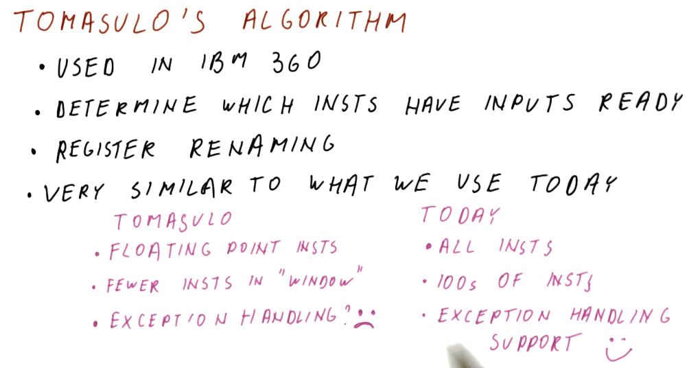
Tomasulo's algorithm is the basis for modern processors' implementation of out-of-order execution. It solves the requirements for register renaming, and is able to determine which instructions have input ready and which instructions are dependent upon pending writes. Below is an excerpt from the class describing what the differences are between Tomasulo's algorithm and how modern processors are designed.

Tomasulo's algorithm - the big picture

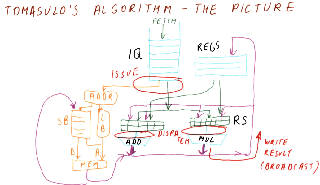
Below is an excerpt from the class drawing out the components that comprise Tomasulo's algorithm. There are a lot of moving parts and they'll be broken down into more detail later - right now we're just summarizing the pieces. Here is a quick description of all of the parts:

• instruction queue - the instruction queue is pretty self explanatory, this is where instructions sit and wait to be issued - they are fetched from memory.
• reservation station - Tomasulo's algorithm was designed for floating point instructions, so this is where those types of instructions wait for their required values before being dispatched. The reservation stations are split into simple instructions that require and adder and more complex instructions that might require a multiplier. Reservation stations enable Tomasulo's algorithm to determine which instructions are ready to execute - implementing out-of-order execution.
• registers - once instructions are dispatched from the reservation stations , the values they generate are written (broadcasted) to the registers. Instructions in other reservation stations will be able to acquire their forwarded values so that they can be dispatched as well.

On the left-hand side of this picture, you'll see that there's logic to cover load and store instructions as well. These were not handled by Tomasulo's algorithm, but modern processors now handle all instruction types similar to Tomasulo's algorithm. The results of the load and store instructions are also broadcasted so that other instructions waiting to be dispatched can take advantage of the values before they are written.

There are three stages of Tomasulo's algorithm:

• issue - this is when an instruction is sorted from the instruction queue into either load / store or a floating point instruction.
• dispatch - this is when an instruction is actually executing using processor resources.
• write result (broadcast) - this is when the result of the instruction is written to the registers file for later use by dependent instructions.

Note - the instructions in the reservation stations also have two inputs per station to receive broadcasts. This is to provide dependent instructions with the necessary values to be dispatched as early as possible.

References

1. Lesson 7 Notes

Issuing

Here are the steps that occur for issuing in Tomasulo's algorithm:

• Take the next instruction, in program order, from the instruction queue.
  • This must be done in program order in order for register renaming to work correctly.
• Determine where input for an instruction originates.
  • Are the inputs required located in the register file? Or are we still waiting on an instruction to generate the necessary values? If we need to wait for an instruction, which one? This will utilize a RAT.
• Find a free reservation station of the correct type (addr or mult).
  • If all the reservation stations are busy, no instructions are issued this cycle.
• Put the instruction in the reservation station.
• Tag the destination register for the result of the instruction being issued.
  • This allows instructions who need this result to be able to reference the correct name and identify their dependency.

Issuing example

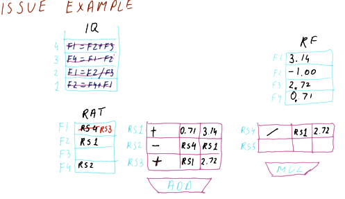
Below is an excerpt from the class that showcases how issuing works. Each instruction is issued from the example instruction queue, and the instruction queue is shifted when an instruction is successfully issued. The are plenty of reservation stations available, so no instructions had to wait in order to acquire a spot in a station.

Following the steps above, before an instruction is issued its inputs must be translated using the RAT. If the value is available, the instruction will read the input directly from the register file. The values that instructions generate will be renamed and the RAT will contain the name of the reservation station for generated values. This way, when other instructions that depend upon a register value are issued, they will use the input generated from other instructions by using their reservation station name.

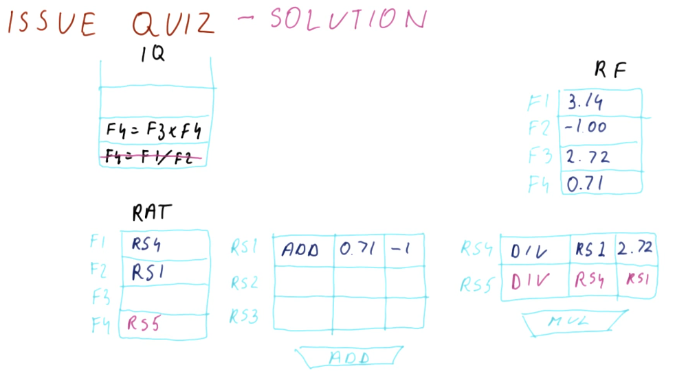
Issue quiz

Below is a quiz from the lectures where we practice the issuing portion of Tomasulo's algorithm. In this example, we are unable to issue the second instruction because there are no spots left in the reservation stations. This example is pretty straightforward.

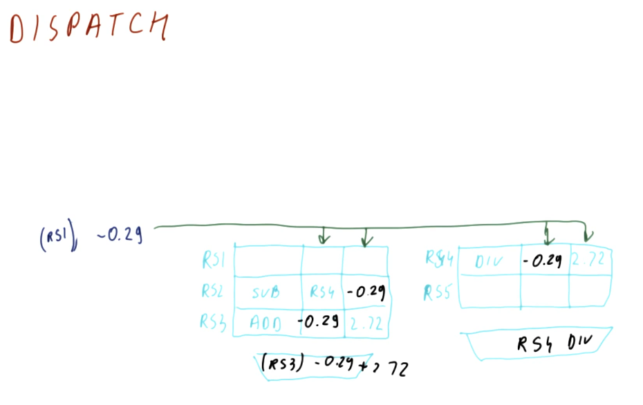
Dispatching

Below is an excerpt from the class that showcases how dispatching works. The results of an instruction from a reservation station is broadcast - its generating reservation station number is attached to the value that it's generating. Instructions that depend upon a value from that reservation station are able to acquire the values necessary to be dispatched, and they will also broadcast their results in the same manner.

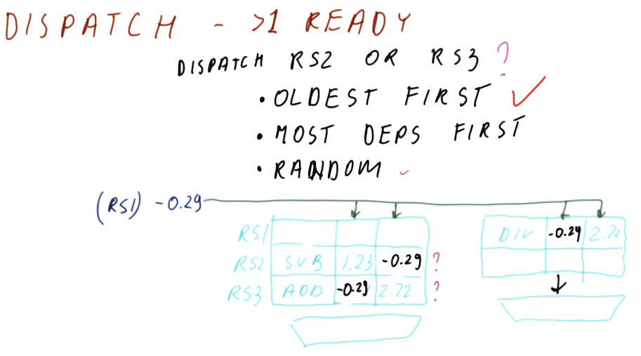
Dispatching when > 1 instruction is ready

Below is an excerpt from the lectures displaying a situation in which more than one instruction in the reservation station is ready to execute. How do we go about making the right decision for best performance? There are three options:

• Dispatching the oldest instruction first - the most fair option and most balanced for performance.
• Dispatching the instruction with the most dependencies - the highest performance option, however, it requires us to search all reservation stations and determine dependencies - power hungry.
• Randomly dispatching - not a bad option, and at some point every instruction will be dispatched, but performance could be degraded.

Dispatch quiz

Below is a quiz from the lectures on dispatching. The quiz asks why the instruction held in RS3 hasn't executed before the current state of the reservation stations. Three options are given, but only two are reasonable.

• The first option: "It was issued in the previous cycle" is reasonable because there can definitely be a time in which the instruction was issued too late so it didn't have time to execute.
• The second option: "Another instruction was dispatched to the adder" is possible because maybe RS1 was currently executing on the adder to generate a value.
• The third option: "RS2 is older than RS3" is not reasonable. The whole purpose of Tomasulo's algorithm is to support out-of-order execution. Instructions will be executed as soon as their values are available, despite how old an instruction is.

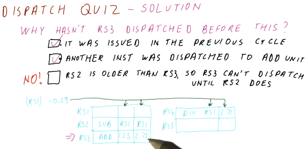
Writing (Broadcast)

Below is an excerpt from the lectures that shows us what happens when a result is written or broadcasted to the reservation stations and the register file. Some steps take place:

• The result is tagged with the reservation station that is generating this result. This combo is then emitted onto the bus.
• The result is written to the register file. We are able to determine what register is being written based upon the RAT - it will contain the name of the reservation station for the appropriate register.
• The RAT is then updated, clearing the reservation station name from the table and marking the location for a register as clear.
• The spot the instruction held in the reservation station is freed.

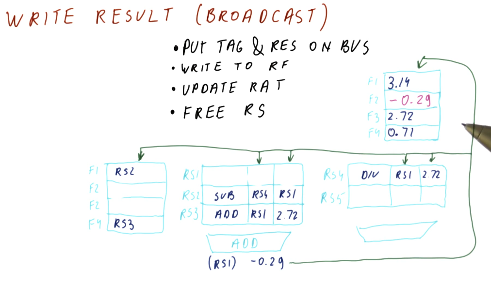
More than 1 broadcast?

There are multiple possibilities that we can consider when handling multiple broadcasts. The first idea is to make more than one bus available - a bus for each dispatch unit in the processor. While that sounds like a good idea, the number of structural dependencies to implement this doubles for each bus - that's a lot of resources and more logic is needed in order to correctly direct the different values being generated.

Another option is to give priority to one dispatch unit over the other, and this is the more likely case. In the example below, we give more priority to the slower dispatch unit. Why? Because if one dispatch unit is slower, it's more likely that faster dispatch units are waiting on values to be broadcasted by the slower one.

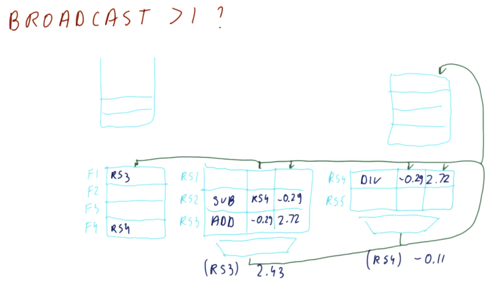
Stale broadcasts

Can we have stale broadcasts? Is that really a thing? Not necessarily. In the example below we see that a broadcast is occurring for RS4, but there's no entry for that reservation station in the RAT. So where will this result be written to - what's its destination?

We can see that RS2 is generating a value and it has overwritten F4, which was the original destination of RS4's value - this is perfectly fine and works as intended. RS2 was the only instruction that depended on the output of RS4, it will have the value it needs to update F4. All subsequent instructions reading F4 will utilize the value generated by RS2 - the "stale" value being broadcasted by RS4 won't cause any issues.

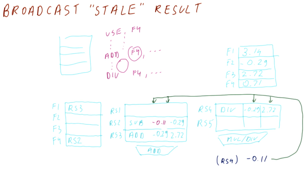
Review

Part 1

Below is a summarization of Tomasulo's algorithm. In this algorithm, for each instruction we are:

• issuing - resolving the registers for an instruction using the RAT and then updating the RAT with the reservation station name of an instruction generating values.
• capturing - capturing output of instructions while in the reservation station.
• dispatching - dispatching ready-to-execute instructions.
• writing results - broadcasting the results of instructions to instructions capturing output in the reservation station, updating the register file and the RAT.

An awesome thing to note as that each of these things is happening for different instructions on each cycle. Every instruction is in one of these stages as we execute instructions out of order.

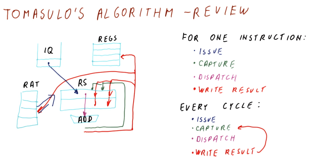
Part 2

Below is an excerpt from the lecture that provides some further discussion of Tomasulo's algorithm. Some questions that are posed:

• Can we issue and dispatch an instruction in the same cycle? - no, we cannot. During an issue and instruction is loaded into the reservation station, we won't be able to dispatch it until we identify that it is ready for executing. While its dependencies may be resolved when being entered into the reservation station, we won't know it's ready to be dispatched until the next cycle.
• Can we capture and dispatch an instruction in the same cycle? - also no, for similar reasons as above. Once an instruction has captured all of its necessary values, it still needs to be marked for execution after the reservation stations have resolved which instructions are ready. This can happen if hardware support is available.
• Can we update the RAT entry for an issue and a broadcast in the same cycle? - yes, the broadcast and the issue can procedures can both update the RAT in the same cycle, however, the issue will be the last to update the RAT. This way, future instructions will reference the output of the reservation station by the issue, not by the broadcast.

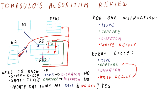
One cycle quiz part 1

Below is a quiz from the lectures where we practice predicting what values will exist in the register file and the RAT after one cycle takes place. In this example we have a processor that does not allow issuing and dispatching in the same cycle, but does allow capturing and dispatching and updating the RAT and writing to the register file in the same cycle.

Given the values provided for the different parts of the scheduler, we are able to determine that the F1 entry in the RAT will be updated by the instruction being issued, and the register file entry for F0 will be updated by the broadcast of RS0. Simultaneously, the entry for F0 in the RAT will be cleared.

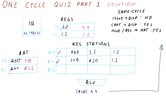
One cycle quiz part 2

Below is a quiz from the lectures where we practice predicting what values will exist in the reservation station for a cycle of the processor pipeline. We can see that an instruction is issued, an instruction is freed from the reservation station upon dispatch, the same instruction that was just issued is able to capture the broadcast of the dispatched instruction.

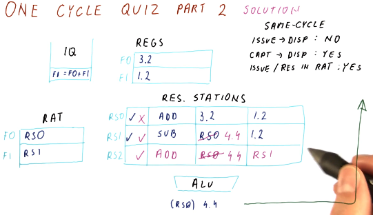
One cycle quiz part 3

Below is a quiz from the lectures where we predict what instruction will be dispatched from the reservation station in the example cycle. We can see that, as soon as the instruction in RS1 captures its required value, it will be dispatched. The instruction in RS2 will not be eligible for dispatch because this processor does not allow issuing and dispatching in the same cycle.

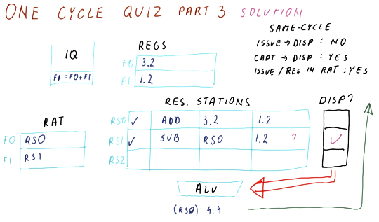
Tomasulo's algorithm quiz

Below is a quiz from the lectures quizzing us on what is not true about Tomasulo's algorithm. What's not true? Tomasulo's algorithm does not dispatch instructions in program order and it does not write results in program order. Tomasulo's algorithm does issue instructions in program order.

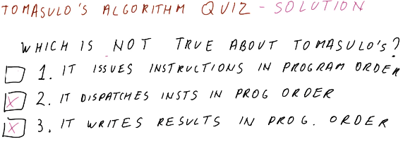
Load and Store

Now that we've discussed how Tomasulo's algorithm handles data dependencies for floating point instructions, how does it handle memory dependencies? Well first, what memory dependencies are there? They're actually the same three categories as data dependencies:

• RAW - an instruction stores a word to some address and then a different instruction loads a word from that same address - this is a true dependency.
• WAR - an instruction loads a word from memory and then another instruction stores a word into memory; if these instructions got re-ordered, we could possibly load the value from the store, thus giving us incorrect program execution.
• WAW - two instructions both write to the same address; if these instructions are re-ordered, it's possible that a stale value is written to the address.

So what do we do about this?:

• In Tomasulo's algorithm, we execute load and store instructions in order. Even if a load instruction is ready to execute, it will be stalled until the store instruction preceding it is completed - even if that store instruction is stalled waiting on some value.
• Modern processors identify dependencies, re-order load instructions, etc. similar to how floating point instructions are handled by Tomasulo's algorithm. These techniques will not be discussed in this lesson, however, they will be touched upon later.

Timing

Below is a quiz on timing from the lecture. Now that we understand the inner working of Tomasulo's algorithm, we predict how long it takes for instructions in the queue to execute based upon the rules provided.

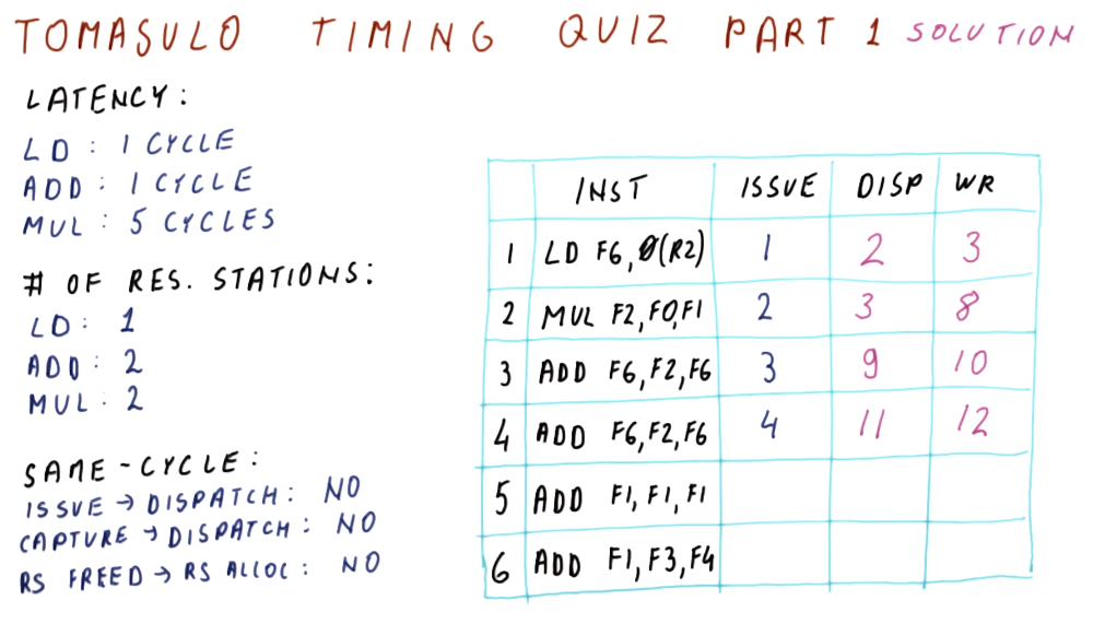
Timing quiz part 2

Below is the second part of the previous quiz. Of note, instruction 5 is unable to be dispatched until cycle 11 because the reservation stations are held by instructions 3 and 4. Instruction 6 cannot be issued until instruction 4 completes its write back and is cleared from the reservation station.

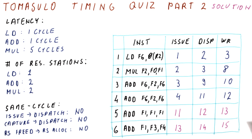
Reorder Buffer (ROB)

Processors can improve performance a lot by reordering instructions. But what happens when the reordering of instructions causes exceptions to happen, like division by zero? This lesson explains how processors cleanup reordered instructions when exceptions happen.

Exceptions in out-of-order execution

Below is an excerpt from the lecture showcasing how exceptions can negatively affect processors that support out-of-order execution. As we can see in this example, instruction 1 takes 40 cycles to complete, however, it encounters an exception where a divide by zero was attempted.

The program counter is saved and an exception handler takes over. After the exception handler executes, the program is restarted from the DIV instruction. Unfortunately, the other three instructions have already executed and have written their results to the registers - thus the DIV instruction will be using the incorrect value for F0 and it will not execute as intended.

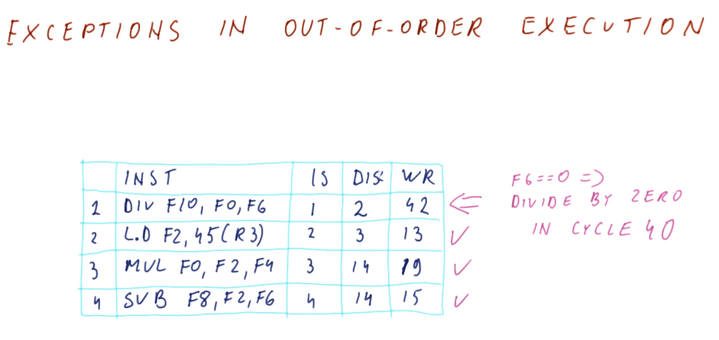
Branch mis-prediction in ooo execution

Below is an excerpt for the lecture covering how branch mis-prediction can also negatively affect our ability to execute instructions out-of-order. In the provided example, the outcome of a DIV instruction determines the jump location for the succeeding BEQ instruction.

In this example, mis-predicting the branch causes us to fetch and execute the succeeding ADD instruction, writing values to R3. Now, when the branch is actually evaluated and executed, we jump to the real landing location of the branch, however, because of ooo execution our value for R3 has been modified incorrectly - succeeding instructions will not execute as intended.

Another example is provided in which we mis-predict the branch and fetch a DIV instruction. This DIV instruction causes a divide by zero exception, but the DIV instruction was never meant to be executed - a phantom exception. The processor goes through all of the steps to handle the exception when, in reality, we were never supposed to execute the DIV anyways.

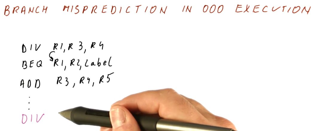
Correct ooo execution

Below is an excerpt from the lectures explain what needs to be done in order to achieve correct ooo execution. We can still execute instructions and broadcast their results ooo, however, we must deposit the resulting values of instructions to registers in order - this is not done by Tomasulo's algorithm which is why we are having problems handling exceptions.

We utilize a mechanism called the reorder buffer that remembers program order, even after the issue stage, and keeps results of instructions until it is deemed safe to write these results to registers.

References

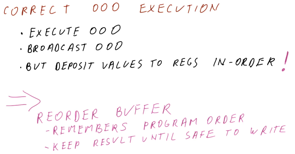
1. Lesson 8 Notes

ROB In Depth

Part 1

The below excerpt from the class gives us a high-level representation of the components of the reorder buffer. The reorder buffer is a table of values, this is what each column represents:

• reg - the target register for writing
• val - the result of an instruction
• done - determines if the data contained in the value column is valid for writing

The reorder buffer also uses two pointers for commit and issue, helping to maintain the results of the instructions in program order. As new instructions are issued they are enqueued into the buffer using the issue pointer. The commit pointer points to the oldest instruction that will be written to its respective register. The instructions between the commit and issue pointers have been deemed valid for writing.

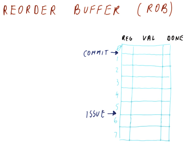
Part 2

The below excerpt from the lectures shows, in detail, how the ROB mechanism is appended into Tomasulo's algorithm to support handling exceptions for ooo execution.

The changes that are made to the algorithm are:

• During an issue operation, the RAT now uses the name of the ROB entry for a register instead of the reservation station.
• During a dispatch operation, the reservation station can be immediately freed because the results of the operation will be using the ROB name instead of the reservation station name.

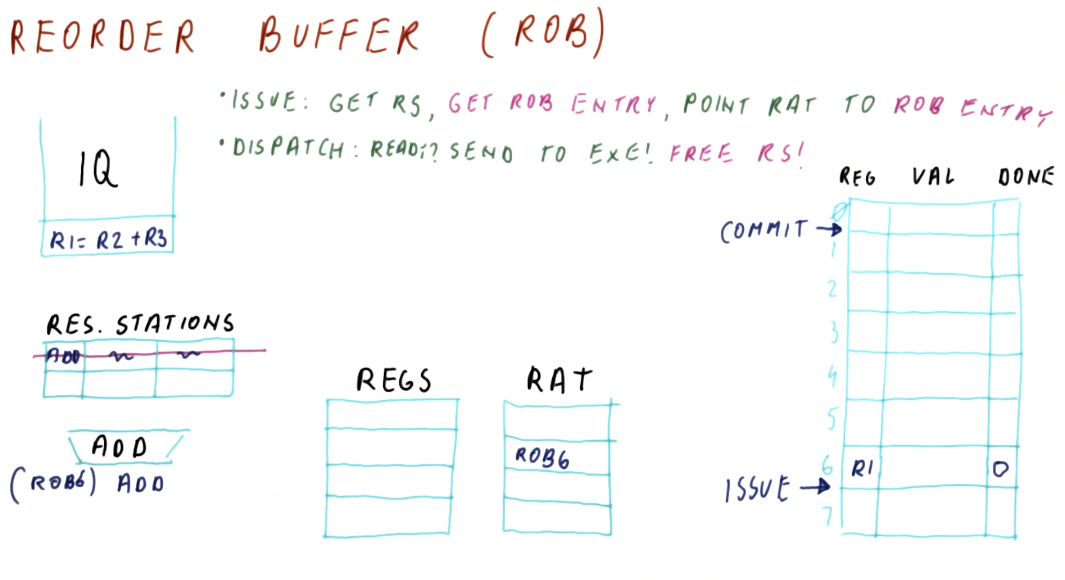
Part 3

The below excerpt from the lectures explains the changes between Tomasulo's algorithm with and without the ROB and how the ROB supports ooo execution with exceptions.

The changes that are made to the algorithm are:

• During the write back or broadcast operation, the values are still captured by instructions waiting in the reservation stations. However, instead of writing the values to the registers and clearing the RAT like normal, the values are written to the ROB, and the RAT maintains its name value for the ROB entry.
• A fourth operation is appended called commit. In the commit stage, we write the value of the register pointed to by the commit pointer, and we update the RAT to point to the newly written register instead of the ROB entry.

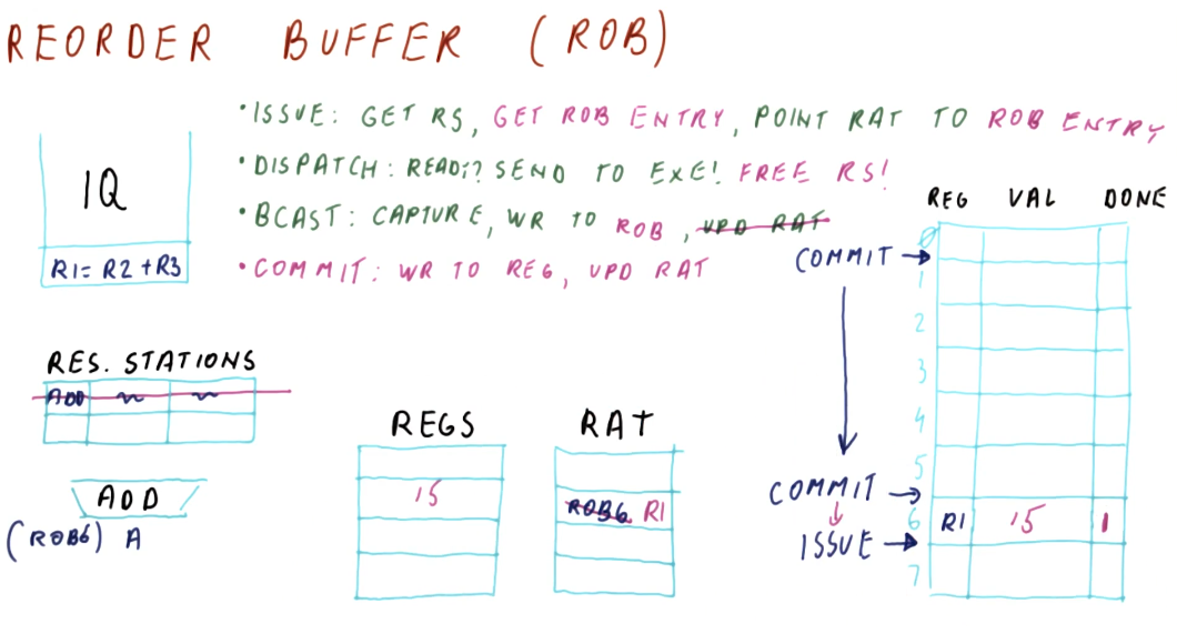
Recovery

Branch mis-prediction recovery part 1

The below excerpt from the lectures provides us a scenario in which a branch mis-prediction occurs and the use of a ROB allows us to avoid writing incorrect values to the registers. Because the instructions in red were never supposed to execute in the first place, we avoid making mistakes.

The example gives us a step-by-step view of how values are updated in the RAT and ROB when each instruction is issued, dispatched, and its values are broadcasted.

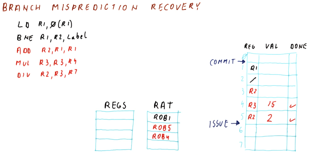
Branch mis-prediction recovery part 2

The below excerpt from the lectures further discusses what takes place when we recover from branch mis-predictions using a ROB. In this example, we can see that these steps are taken to fully recover from a mis-predicted branch:

• The RAT is cleared and points back to the values contained in the registers
• The ROB is "emptied" by resetting the issue pointer to the commit pointer
• The reservation stations and the computational units (ALU / MUL, etc.) are drained until they are empty

The mis-predicted branch is only noticed when the commit pointer in the ROB sees that mis-predicted branch value in the branch's ROB entry.

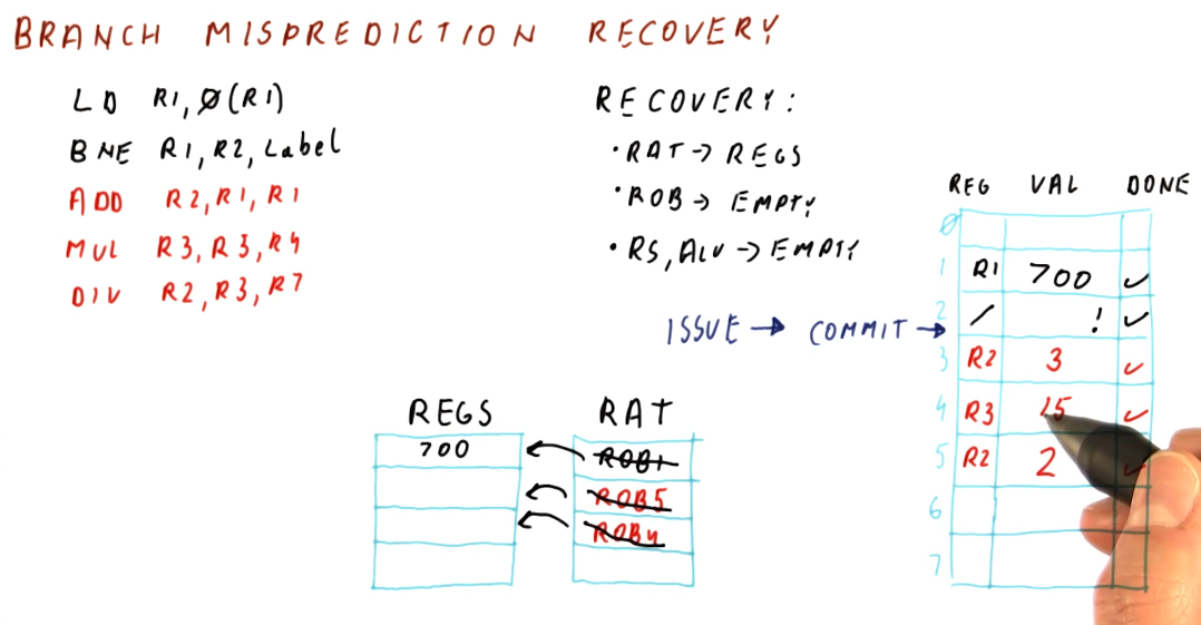
ROB and exceptions

In the below excerpt, we cover how exceptions are handled using ROB. In summary, we treat exception as a result like they would be from any other operation. The exceptional instructions are marked in the ROB and aren't handled until the commit pointer arrives to them in the ROB. We delay the handling of exceptions until they need to be committed - this provides us a good return point for an exception handler and prevents us from writing the results of instructions that took place out-of-order before we noticed the exception. This also resolves the issue of phantom exceptions - if the branch was mis-predicted we will end up ignoring the phantom exception so effectively it never happened.

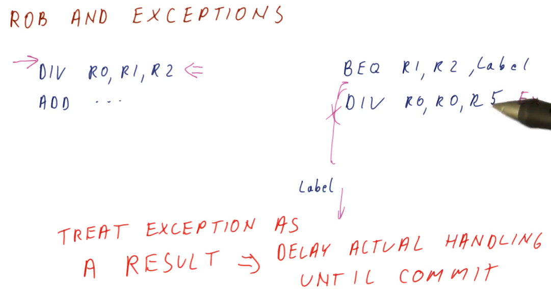
Exceptions with ROB quiz

Below is a quiz from the lectures covering exceptions with ROB. A DIV instruction caused a divide by zero error - to solve the quiz we must predict the new state of the ROB when the exception is noticed.

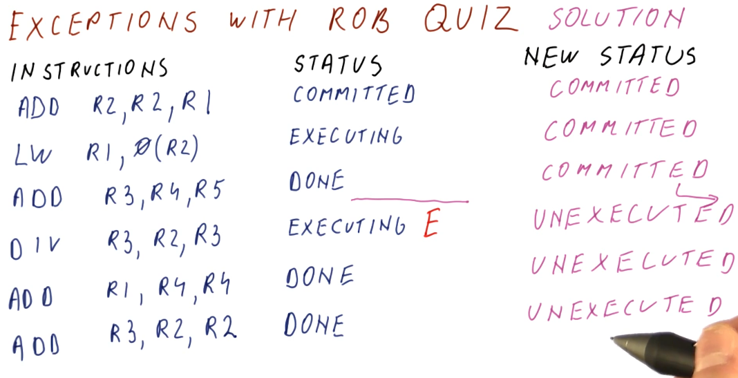
RAT updates on commit

The below excerpt from the lectures showcases how the registers and RAT are updated using the ROB and why. Upon each commit, the values contained in the ROB are written to the registers. The RAT, however, is not cleared or updated until the corresponding ROB entry is committed. This is to help instructions that are being issued to keep track of and use the most recent name for the outcome of a register.

So why are we writing to the registers on each commit? Because, if an exception takes place, all of the changes that are valid are written to the registers and saved. The ROB can safely drain the instructions that aren't meant to be written and the RAT can be cleared and updated to point to the registers.

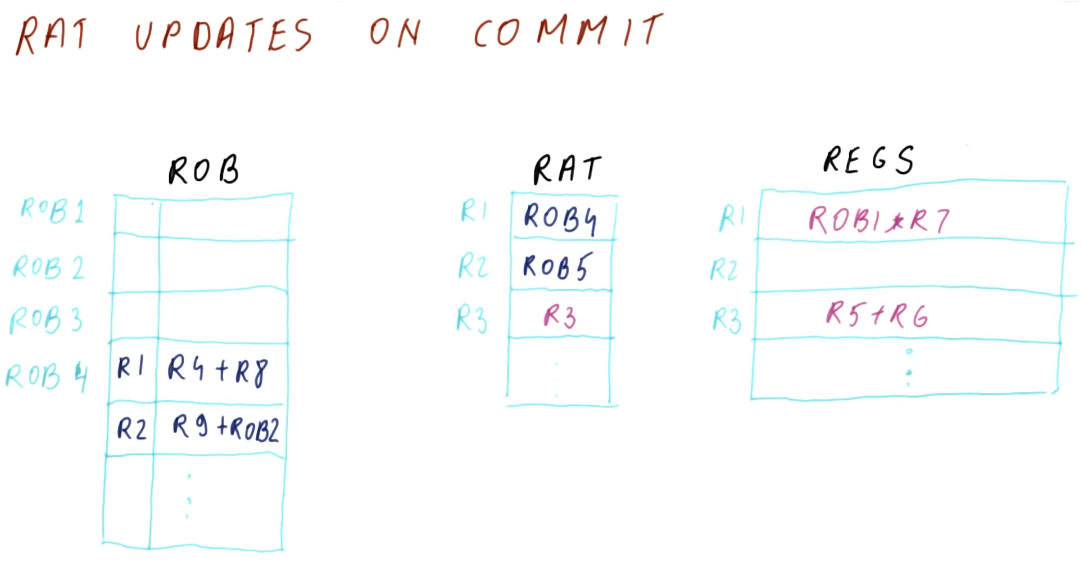
ROB Timing

Below are ROB timing quizzes and examples from the lecture.

ROB timing example

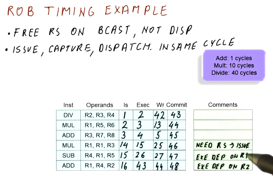
ROB timing quiz

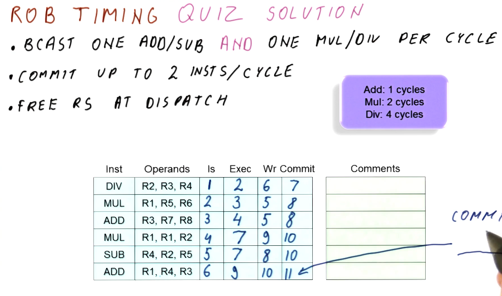
Extra Topics

Unified reservation stations

Unified reservation stations are touched upon in the below excerpt for the class . With unified reservation stations, we gain the ability to issue more instructions because we aren't segregating our instructions into two groups - instructions will now gain a reservation station based on a first-come-first-served basis. This will allow our pipeline to stop less often as well, as we will always be able to make the most of our available space.

A drawback for unified reservation stations is that more logic is required in order to implement this change. We must now include logic in order to sort between which instructions use what structural capability (ADDR or MUL) and we also need to be able to selected two instructions for execution per cycle, one ADDR and one MUL.

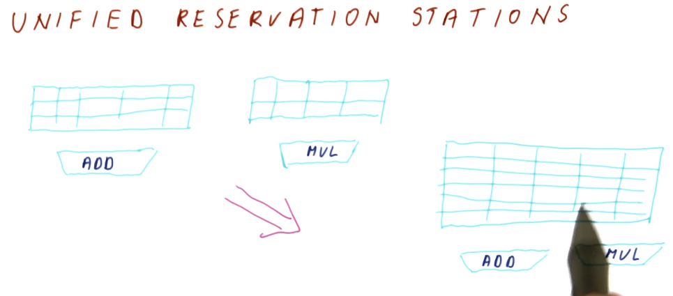
Superscalar processors

The below excerpt from the lectures discusses the requirements to implement superscalar processors. The central takeaway from this discussion is that a superscalar processor will only be as strong as its weakest link. If an operation in this listing presents itself as a bottleneck, our performance will only be as good as that one operation.

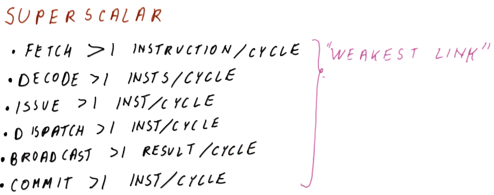
Terminology confusion

This excerpt from the lectures clears up any possible confusion between the terminology used for Tomasulo's algorithm in academia and what terms are used in the industry.

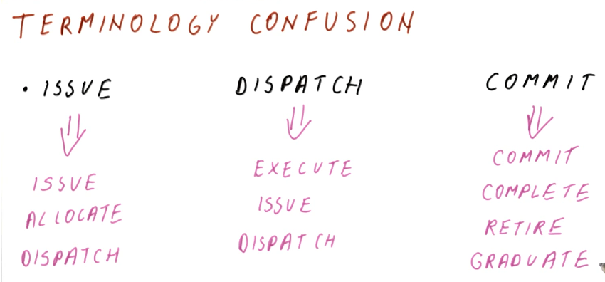
Out of order?

In our recent discussions, we've been issuing instructions one-by-one. What is really out of order in Tomasulo's algorithm that provides us a performance increase? The below excerpt from the lectures further discusses this.

The central takeaway is that these portions of the pipeline have this behavior:

• Fetch, decode, and issue stages happen in program order in order to identify and resolve dependencies.
• Execute and write result (broadcast) stages happen out of order.
• The commit stage happens in program order to give the appearance externally that we are executing instructions in program order.

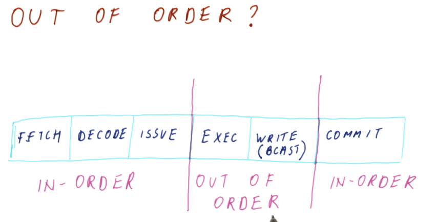
In-order vs out-of-order quiz

The below excerpt is a quiz from the lecture requiring us to identify what parts of the pipeline are conducted in program order.

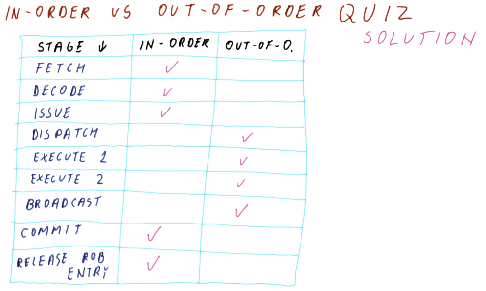
Memory Ordering

In previous lectures we have seen that processors conducting out-of-order execution can track when instructions use registers populated by preceding instructions. In contrast, load and store instructions can reference values located in memory, so how does a processor de-conflict load and store accesses to values in memory when conducting out-of-order execution?

The notes for this lecture can be found here

Memory access ordering

So we've already demonstrated that we can resolve control dependencies by implementing good branch prediction. We have eliminated false data dependencies for registers using register renaming. We have also shown that out-of-order execution can respect RAW or true dependencies by using Tomasulo-like scheduling of instructions in reservation stations.

The two techniques we have used to eliminate data dependencies are only applicable to operations involving registers. We still have to resolve dependencies that manifest when conducting load and store instructions on the same locations in memory. How do we execute these instructions out-of-order?

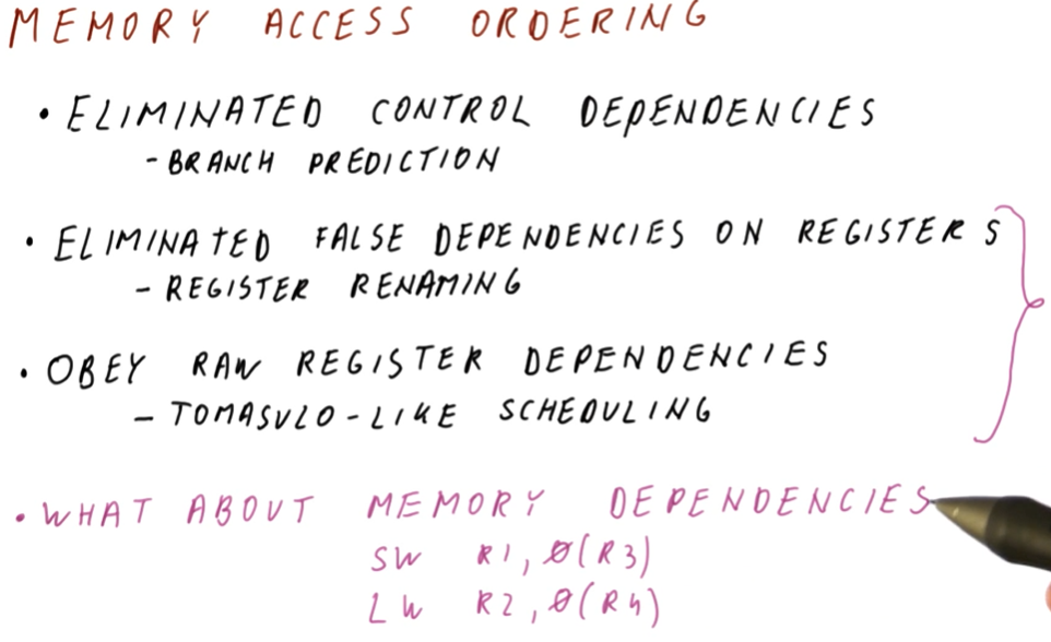
Memory writes

For store instructions, knowing when memory writes actually happen is important. Memory writes actually happen when an instruction commits. Memory writes only happen when a commit takes place for an instruction because it is dangerous to do so, otherwise. If we wrote to memory prior to an instruction committing, that information could be written but the instruction could be cancelled due to something like branch mis-prediction or an exception.

To resolve this issue, we delay memory writes and stores until the instruction is committed.

So where and when do load instructions get their data? We want load instructions to get their data as soon as possible. Do they always have to wait until every store instruction commits?

To resolve this issue, computer architects implement a load-store queue structure to keep all load and store instructions. More on this in the next section.

Load-Store Queue (LSQ)

The load-store queue is similar to the ROB. This queue contains load and store instructions in the sequence in which they will be committed. The fields are as follows:

• l/s - bit that identifies whether the current entry is a load or store instruction.
• addr - the address the instruction is accessing.
• val - field for the value that the instruction should be loading or storing.
• c - marks if the entry has been committed.

The load-store queue also implements a mechanism called store-to-load forwarding. If a load operation has a matching store operation preceding it, meaning the load operation in question is loading from a previously written memory location, we can forward the value of the preceding store operation in the queue to the load operation in the queue. This affords us the ability to avoid having to access memory at an already written to location - we already know the value it contains thanks to the queue.

Below is a high-level representation of the concepts discussed above.

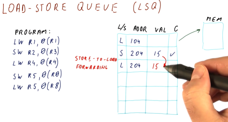
Load-Store Queue part 2

So what happens when we have a load instruction and we know the target address , but we didn't previously store to this location so we don't know the value for forwarding purposes? We have three options that have been considered:

• in-order - in this case, we execute all the instructions in order to ensure the fidelity of the contents of our target address. This defeats the purpose of our discussion as we want to conduct out-of-order execution - we want all the load instructions to execute as soon as possible.
• wait for all stores - in this case, we wait for all previous store instructions to execute before executing our load instruction.
• go anyway - the most aggressive option - we execute the load instruction as soon as we resolve the target address.

Two things can happen for the go anyway option:

• Previous store instructions will resolve their target addresses and we determine that it was safe for us to load from our target.
• Previous store instructions resolve their target address and we realize that the target was supposed to be written to before we executed our load instruction. Thus, we've loaded an incorrect value from memory and we need to recover. In this case, store instructions will check if any load operations succeeding them match their target address. If so, if they are marked complete in the queue, the store instruction will mark them incomplete.

Most modern processors use the go anyway option as they produce the best performance.

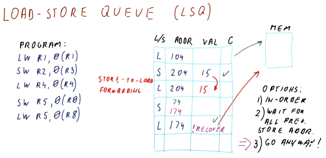
Store to load forwarding

Some central questions need to be answered for store-to-load forwarding. Below is the lecture snapshot containing these questions.

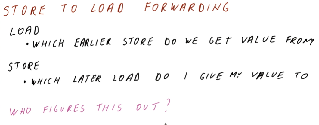
LSQ example

Below is a more detailed representation of the load-store queue.

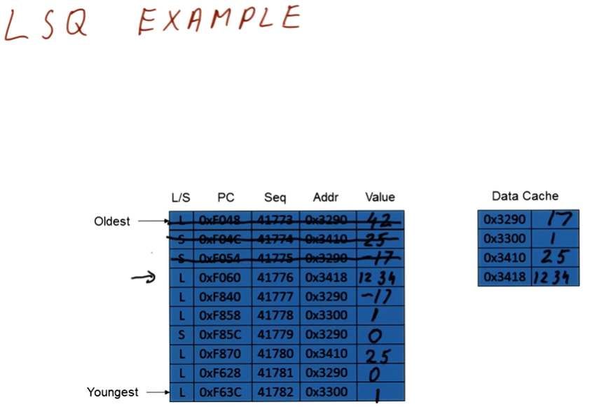
OOO Load/Store Execution

The below example discusses the intricacies of out-of-order execution of load and store instructions. In the example provided, the sub operation is able to execute out-of-order because it has no dependencies. Once it produces a value for R1, we execute the dependent load instruction. Meanwhile, the first load in the queue encountered a cache miss and is waiting memory addressed by R6 to be loaded.

When the first load instruction finally completes, the dependent store instruction resolves its target address with the previous add and notices that the succeeding load also target the same address. Thus, the succeeding load instruction loaded a stale value from memory and the instructions in the queue need to be invalidated.

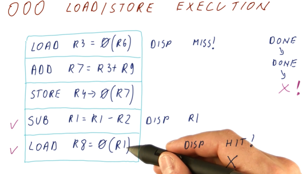
In-order Load/Store Execution

In contrast, an example is provided for in-order load and store execution of the load/store queue. It discusses how we can dispatch non-load and non-store instructions for execution if they contain no dependencies. However, this model still enforces that load/store instructions execute in order so, even if we have our target address calculated, all preceding store instructions must commit before we can load.

In this example, the first load instruction encounters a cache miss and also resolves a dependency for the preceding arithmetic operation. Thus, the succeeding store operation is also stalled. The sub operation further down in the queue is able to be dispatched out-of-order, the load operation, however, cannot proceed because the previous store operation has not taken place.

While this may avoid us having to recover if the last load reads stale values, this also prevents us from leveraging a performance increase if the last load didn't actually depend on the preceding store.

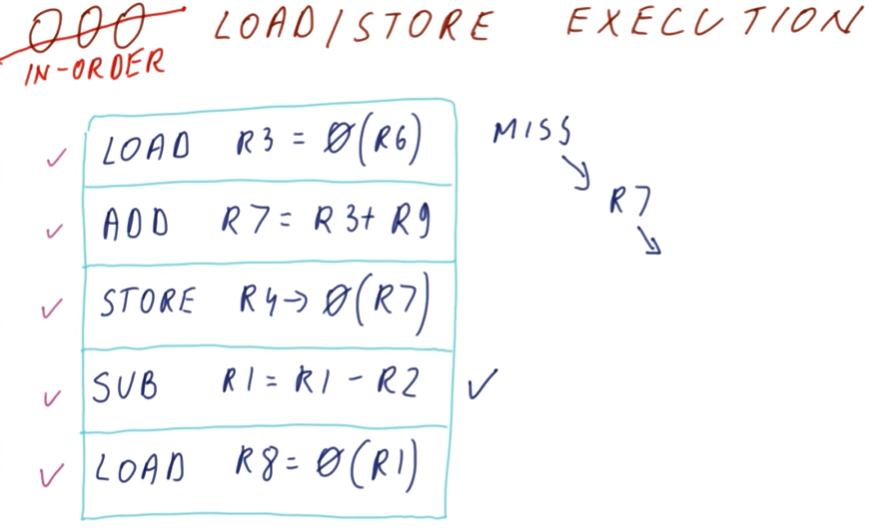
Memory ordering quiz

In this quiz we are instructed to determine how many cycles it would take to execute the instructions in the provided load-store queue in-order if all load instructions encountered a cache miss of 40 cycles.

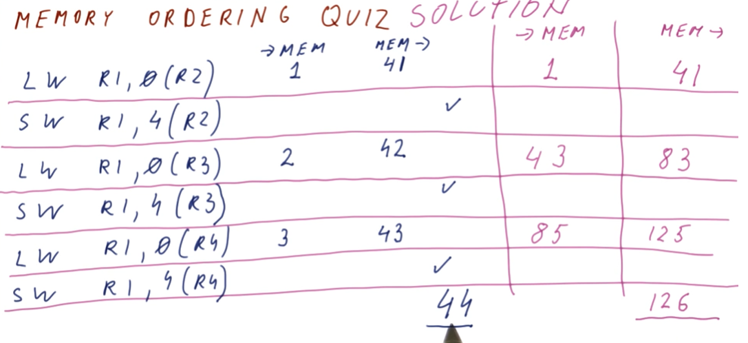
Summary

LSQ, ROB, and RS

So how do the load-store queue, reorder buffer, and reservation stations (RS) play together in our out-of-order processor? The notes from the lecture below provide a high-level discussion.

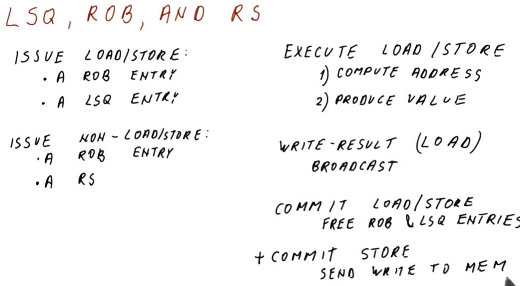
Memory ordering quiz

Below is a quiz from the lectures wrapping up our understanding of where load instructions acquire their values using a LSQ.

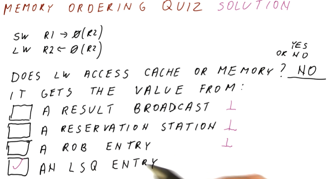
Compiler ILP

In previous lessons we discussed out-of-order execution processors that attempt to execute more than one instruction per cycle. In this lesson we will discuss how compilers can support this process.

The notes for this lecture can be found here.

Can compilers improve IPC?

At the processor level, we face a couple of obstacles that prevent us from further improving our IPC and performance. These include:

• dependence chains - a program can contain dependency chains that could otherwise not exist if a compiler were to remove the dependencies and use other registers for storing information.
• limited "window" into the program - a processor can only see so many instructions at once. Independent instructions that could be executed concurrently could exist far from each other in the program, not leveraging the out-of-order execution capability of the processor.

Below is a high level representation of the concepts discussed above with some pseudo-assembly.

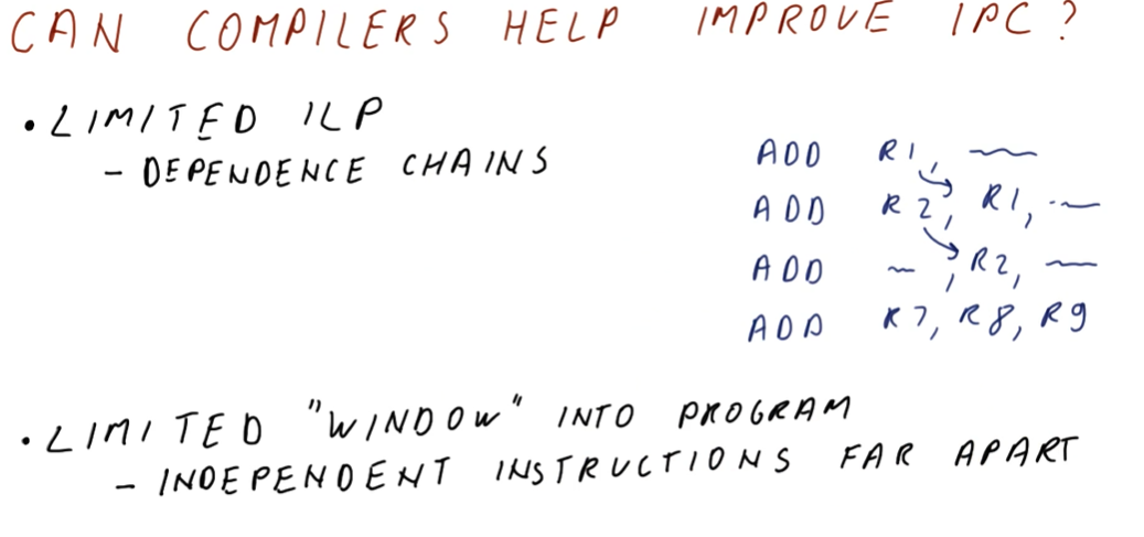
Tree Height Reduction

Using Tree Height Reduction, compilers remove dependency chains from the program by identifying operations than can be conducted concurrently and separating them. In the example below, our code wants to store the summation of four operands into the register R8. Without Tree Height Reduction, our code would create a dependency chain as we execute sequential instructions to add to register R8. With Tree Height Reduction, the compiler groups the operations and removes the dependency by using another register, R7, to hold the intermediate value.

We aren't able to use Tree Height Reduction all of the time as it uses associativity. If an operation isn't associative, Tree Height Reduction cannot be applied.

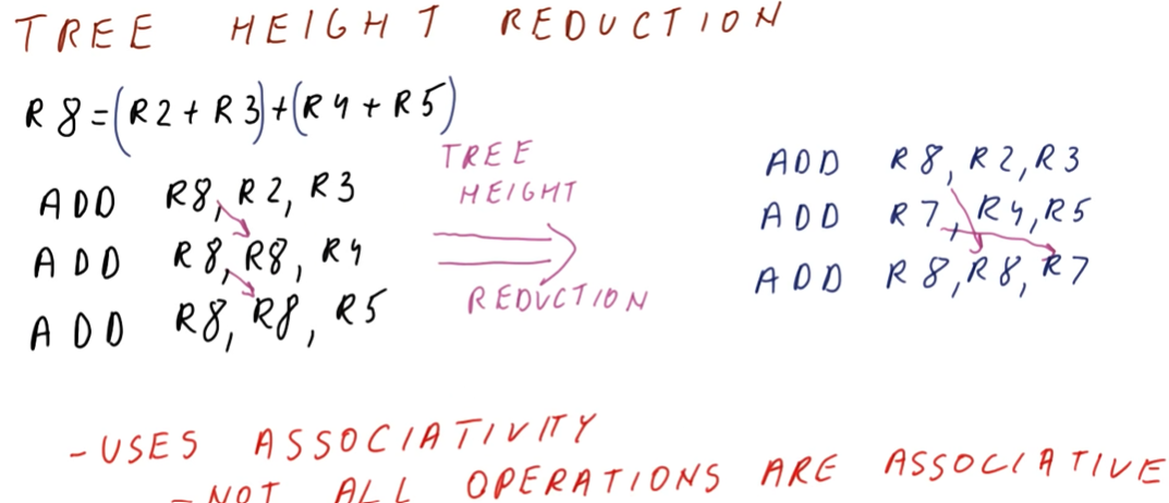
Tree Height Reduction Quiz

Below is a quiz from the lectures showcasing how to conduct Tree Height Reduction with a set of assembly instructions. To solve the quiz, we must reconstruct the original expression from the assembly instructions. Then we group together the ADD operations and get the final value for all of the positive numbers. Next we group together all of the negative numbers with ADD operations, and then we subtract the two summations.

Once we identify all of the dependencies in the reduced assembly code, we can see that the new code is able to execute more instructions out-of-order, and we double our ILP.

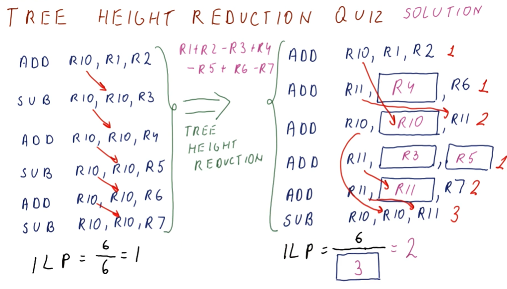
Instruction Scheduling

The idea behind instruction scheduling is to identify instructions that will take a couple of cycles to complete and moving instructions that take less cycles to complete to "stall" locations in the program. This way, we can execute non-dependent instructions while waiting for something else to happen, like a read from memory.

The excerpts below provide a high-level representation of a how a compiler identifies stalls in the program code for long operations and rearranges instructions to leverage as much concurrency as possible.

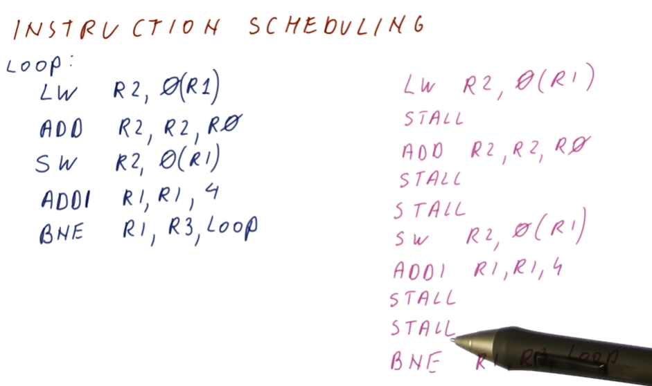
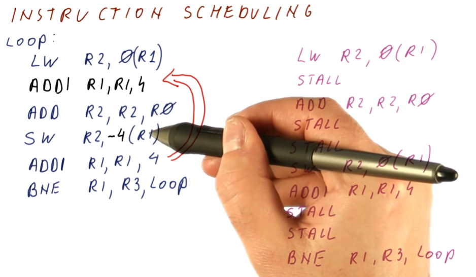
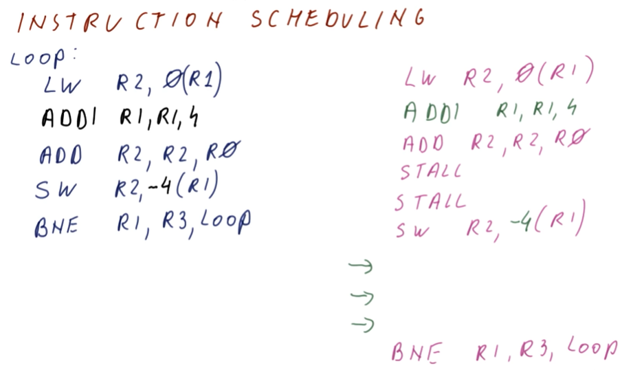
Instruction Scheduling Quiz

The quiz below showcases how we can use instruction scheduling to decrease the number of cycles it takes to complete a series of instructions. Without instruction scheduling, it takes us 8 cycles to complete the series of instructions. Once we identify the stalls, we see that we can execute the second LOAD operation right after the first one if we rename the target register from R1 to R10.

With instruction scheduling, we are able to execute the example instructions in 6 cycles.

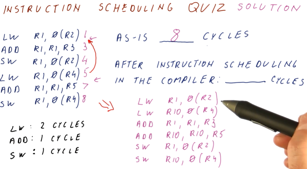
Instruction scheduling and If conversion

We can easily apply instruction scheduling to the blocks of code in different branches, but how do use instruction scheduling across blocks of code in different branches? If we conduct instruction scheduling without predication, we would move some instructions in to different branches, however, if that branch does not execute, the re-scheduled instruction does not get executed, changing the behavior of the program.

To solve this, we can combine the branches using predication. We prepend the code of if-else statements with predicates, combine the branches into one block, and execute all instructions. Then we apply instruction scheduling to increase our efficiency.

Below is a high level representation of this concept.

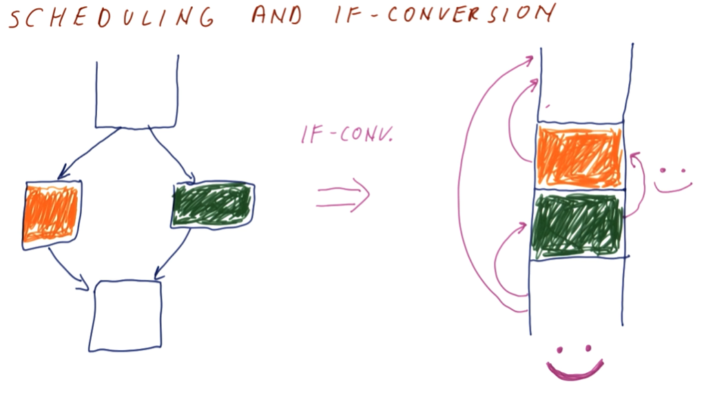
Loops and If conversion

So, can we conduct instruction scheduling on loops, using If conversion and predication to enable the movement of instructions in the program? Yes, instruction scheduling can be done on the block of instructions that comprises a loop, however, in order to remove the branch instruction to conduct If conversion, we would have to install predicates for each loop of the branch. Is this feasible? Absolutely not - what if we had a branch that looped a million times, would we install a million predicates?

Below is an excerpt from the lecture explaining this issue at a higher level.

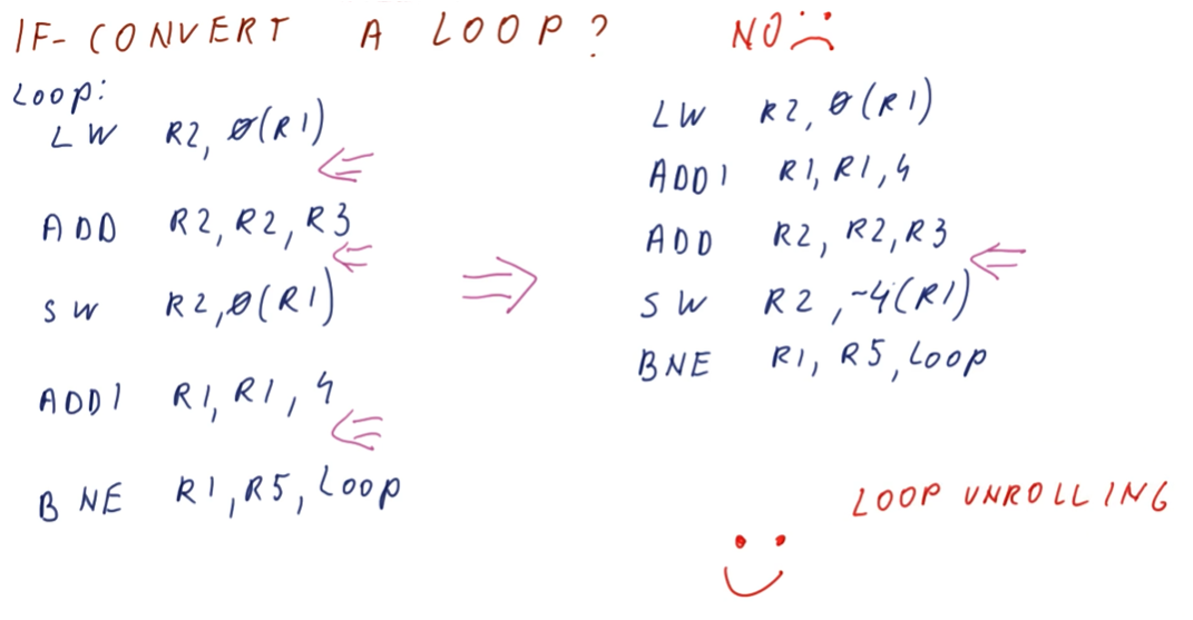
Loop Unrolling

So how do we get better performance out of loops? Well, we do more work per loop iteration. In Loop Unrolling, the compiler identifies what work is done each loop and sees if it can execute more instructions per loop iteration. In the example provided below, the program adds a number to each element in an array. With Loop Unrolling, the compiler unrolls the loop once and executes the addition of the variable to the next array item in the loop. The loop iterator is also decremented by 2 instead of 1 to compensate for these changes.

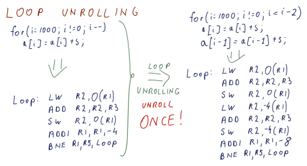
Loop unrolling benefits: Instructions

Loop Unrolling provides us a benefit - we can do less instructions per loop evaluation! In the example below, we compare two loops, with one being the unrolled loop.

When evaluation the unrolled loop, we actually execute less instructions because we execute the last two instructions, ADD and BNE, less times! These instructions are what's known as the loop overhead.

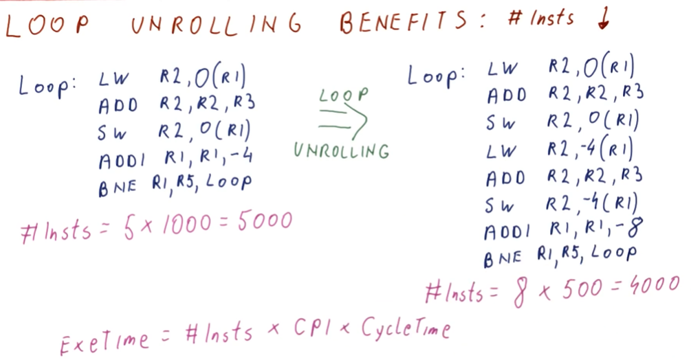
Loop unrolling benefits: CPI

Below is the breakdown of CPI for a branch before and after instruction scheduling is applied. Re-scheduling the instructions, we see that we can avoid waiting unnecessary cycles for an operation to complete when other operations that aren't dependent on previous instructions can be dispatched.

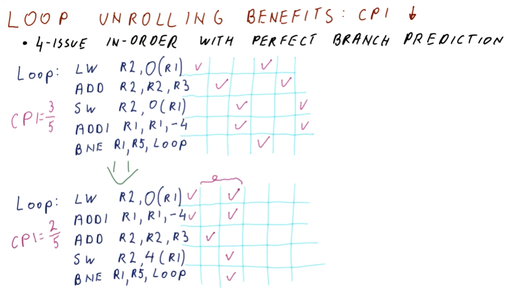
The excerpt from the lectures below now does a comparison of the example loop above, however, we have unrolled the loop once. The unrolled loop without instruction scheduling doesn't see much of a performance increase. Yes, we execute less instructions because we've unrolled the loop, however, because the instructions aren't scheduled we have to wait a couple of cycles for dependencies to be resolved.

Contrast this with the unrolled, re-scheduled loop. We use another register, R10, to hold the contents of the next item in the loop at R1 - 4. We also re-schedule the add instructions because they are only dependent upon the loads. The add instruction from the loop overhead can also be conducted in parallel because it has no dependencies. Finally, our STORE instructions are edited to compensate for the changes made to R1.

Because of this, we can see that our CPI decreases greatly and we are able to leverage parallelism.

Unrolling downsides

Below is an excerpt from the lectures containing a high-level representation of the downsides to loop unrolling. Here's a breakdown:

• code bloat - depending on how many times we unroll the loop, we can bloat the size of the code in the program.
• unknown number of iterations - what if we don't know the number of iterations? How would would be able to effectively unroll a loop? With an unknown number of iterations, we could exit the loop early and not execute the rest of the unrolled loop - which is an issue.
• number of iterations if not a multiple of N - what if we're doing an odd number of iterations and we didn't unroll the loop to fit this? We need to exit the loop early without executing the rest of the unrolled loop - how do we make that happen?

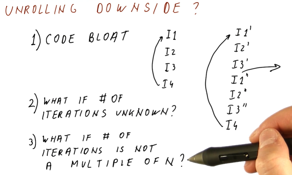
Function Call Inlining

In Function Call Inlining, the compiler identifies simple functions that can be inlined into the rest of the program code. The example below shows a simple function that executes one instruction and then returns. This function is wasteful each time it calls because we have to setup its arguments, call, and then return - it's unnecessary overhead.

Function Call Inlining eliminates call and return overheads because the code is in the same location. This also allows us to leverage instruction scheduling because the code is no longer segregated due to function semantics. We are able to leverage this combination of performance enhancing measures to gain a shorter execution time.

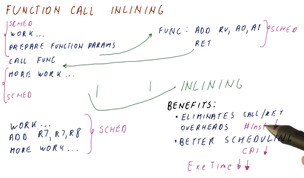
Function Call Inlining Downsides

Function Call Inlining is subject to code bloat, just like loop unrolling. In the example provided below, we have a function that is comprised of 10 instructions. If the function is inlined for each instance it is called, we would end up repeating the same 10 instructions in the program a bunch of times. We can see how the program code might increase by a large amount if we inlined a function that was called a lot of times.

We have to be judicious about which functions are inlined. They need to contain small amounts of code, and it probably makes sense to ensure they aren't called often.

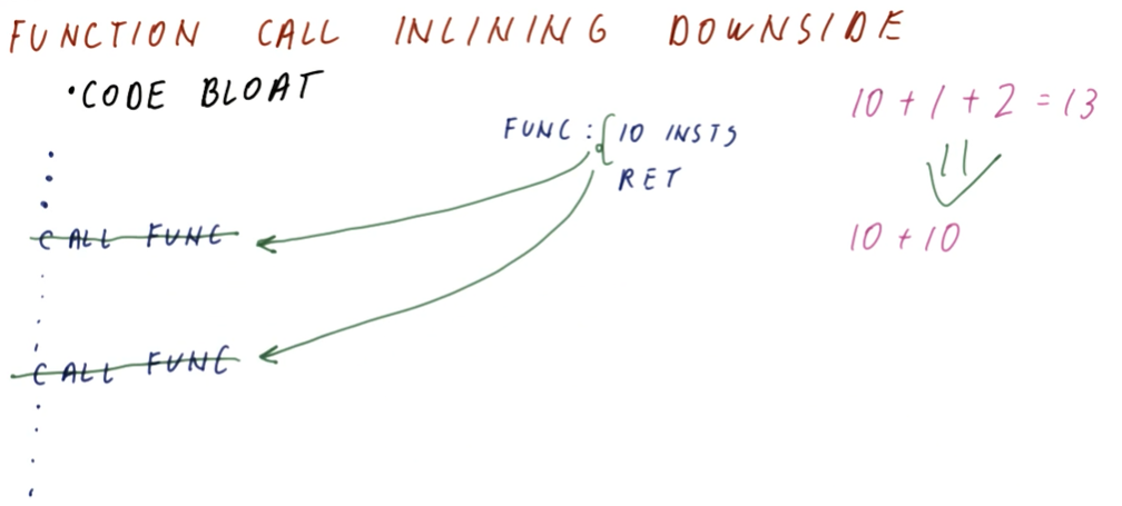
Function call inlining quiz

Below is a quiz from the lectures. In this quiz, we compare the number of cycles it takes to execute a block of code, with and without function call inlining. In this example, there's no real way we can conduct instruction scheduling due to the dependencies of the instructions, however, we increase our performance and execute less cycles when function call inlining is implemented because we avoid executing the CALL and RET instructions.

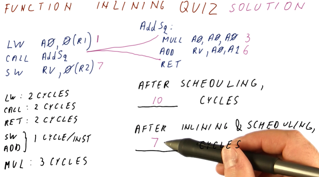
VLIW

This lesson covers VLIW and explicitly parallel processors. These processors do not try to identify ILP on their own, instead doing what the compiler instructs them to do.

The notes for this lesson can be found here

Superscalar vs VLIW

Below is an excerpt from the lectures describing the differences between out-of-order and in-order superscalar processors and very long instruction word (VLIW) processors.

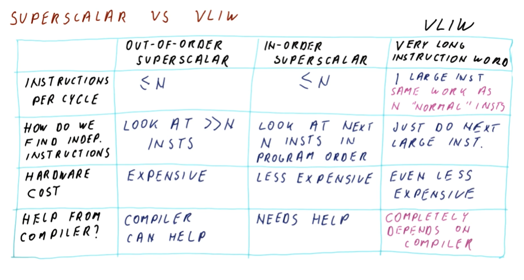
Superscalar vs VLIW quiz

Below is a quiz from lectures comparing the possible program size between a out-of-order superscalar processor and a VLIW processor. If each 128-bit instruction for a VLIW processor has no dependencies and can execute all four operations at once, our programs can be equivalent. If we have dependent instructions, however, there's a worst-case possibility our 128-bit instructions would include NOPs for 3/4 operations. This would quadruple the program size.

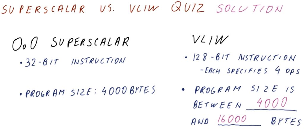
VLIW: the good and the bad

Below is an excerpt from the lectures providing a high-level description of the pros and cons of VLIW processors. A quick breakdown of what's not covered in the image below:

• Compiler does the hard work - plenty of time. The basic discussion around this is that the compiler has more time to schedule instructions, and the program will be run many times afterwards. This is in contrast to superscalar processors that must schedule instructions during runtime.
• Latencies not always the same - this is talking about how the compiler won't be able to predict how much latency will be present when the code executes on different hardware. Cache misses might take longer in different environments.
• Irregular applications - it's difficult for a compiler to schedule and predict the semantics of an irregular program. Things that leverage machine learning, etc. are in this group.

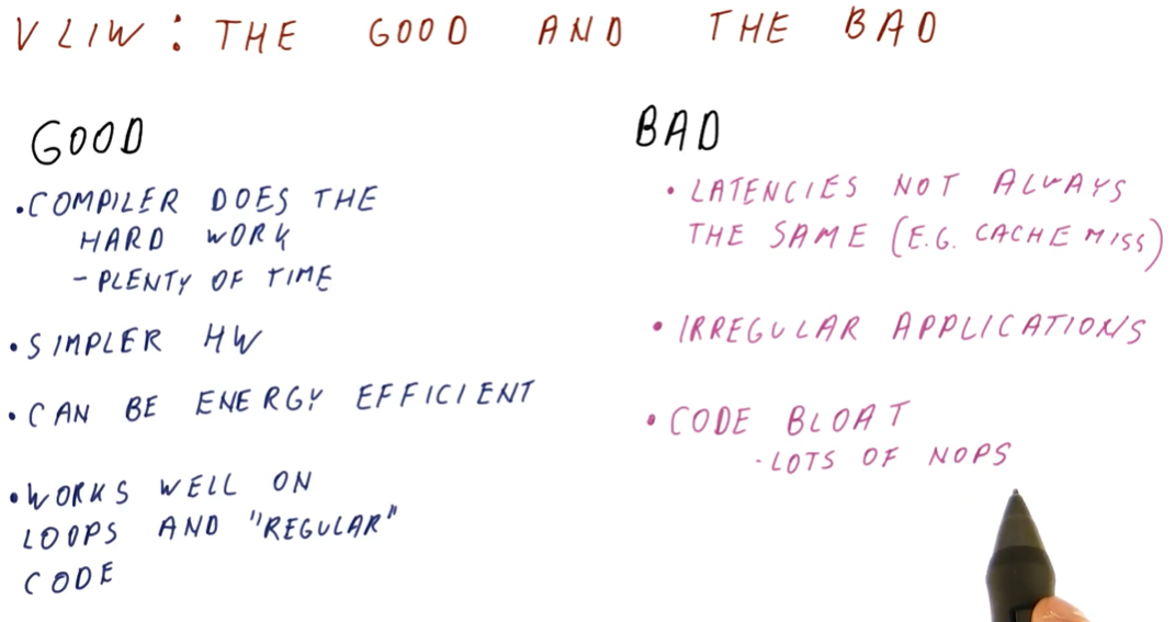
VLIW backwards compatibility quiz

Below is quiz about VLIW backwards compatibility. In this instance, the new compiler is not a VLIW processor. Why? With VLIW, the compiler guarantees that an instruction contains multiple independent operations. If we increase the number of instructions executed per cycle, we cannot guarantee that dependencies will not exist between the two instructions being executed - the compiler did not account for this and we're breaking the contract, anyways.

In order to run a program on this new VLIW processor, we need to re-compile the code so that the compiler can re-schedule the instructions and resolve dependencies.

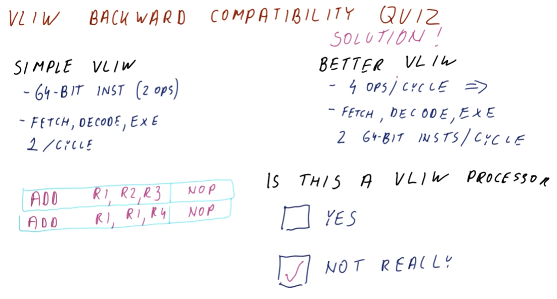
VLIW instructions

Below is an excerpt from the lecture, describing the the characteristics of VLIW instructions.

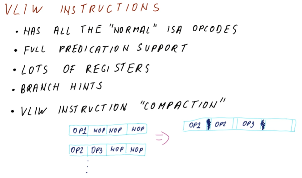
VLIW target market

Below is quiz from the lectures asking us to rank the best application for VLIW processors.

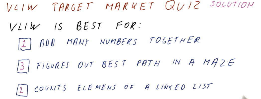
Cache

This section conducts a review of the hardware cache. The notes for this lesson can be found here

Locality

Below is a high-level description from the class describing the concept of locality.

The below image from the lectures describes the concepts of temporal locality and spatial locality.

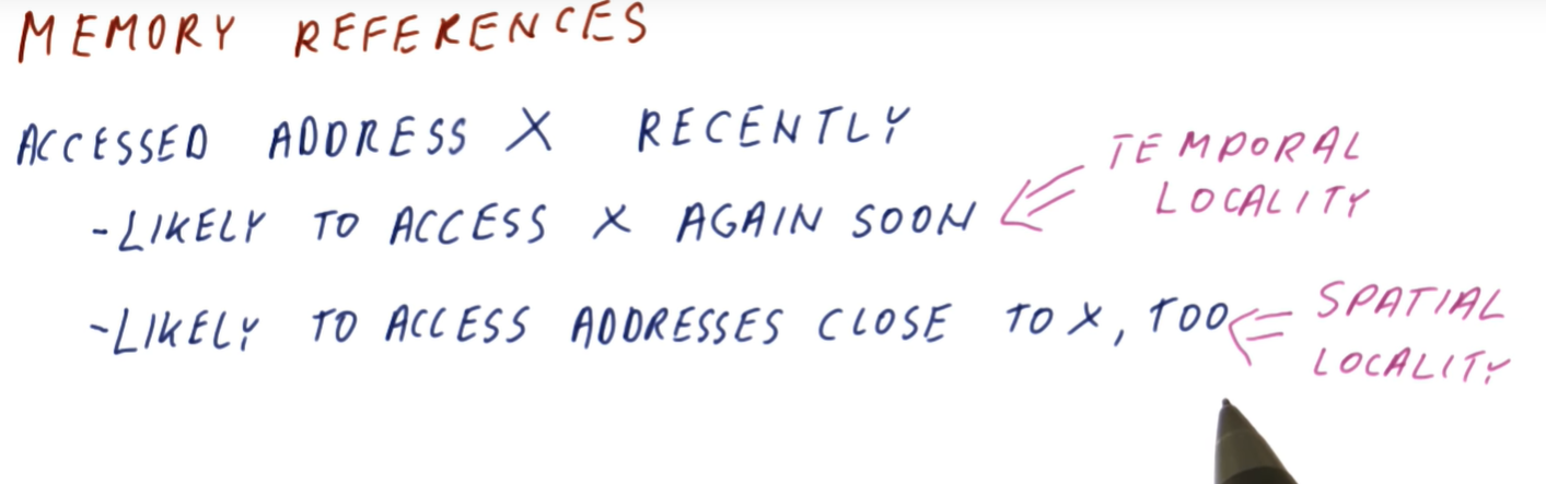
Temporal Locality Quiz

The below quiz from the lectures discusses temporal locality with an example section of code. The j and sum variables are accessed very often, having temporal locality in the cache.

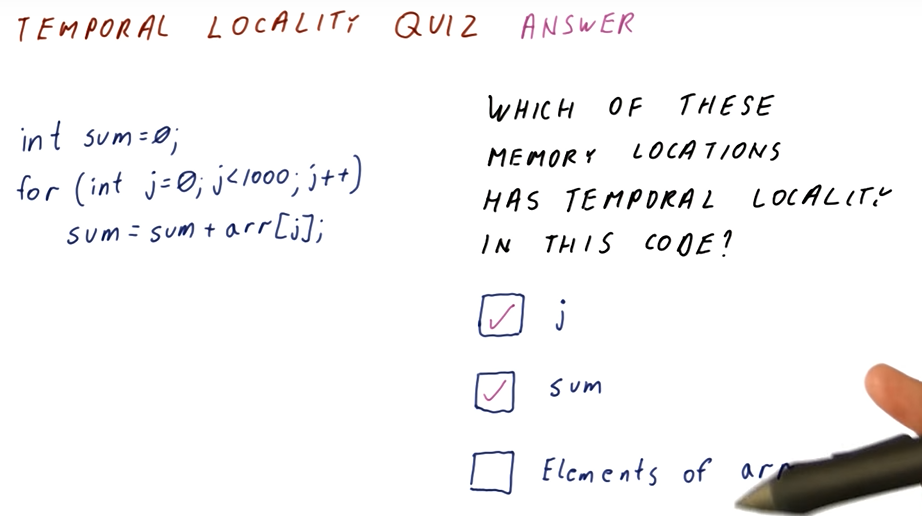
Spatial Locality Quiz

We are likely to access all elements of the array in this loop, thus arr has spatial locality.

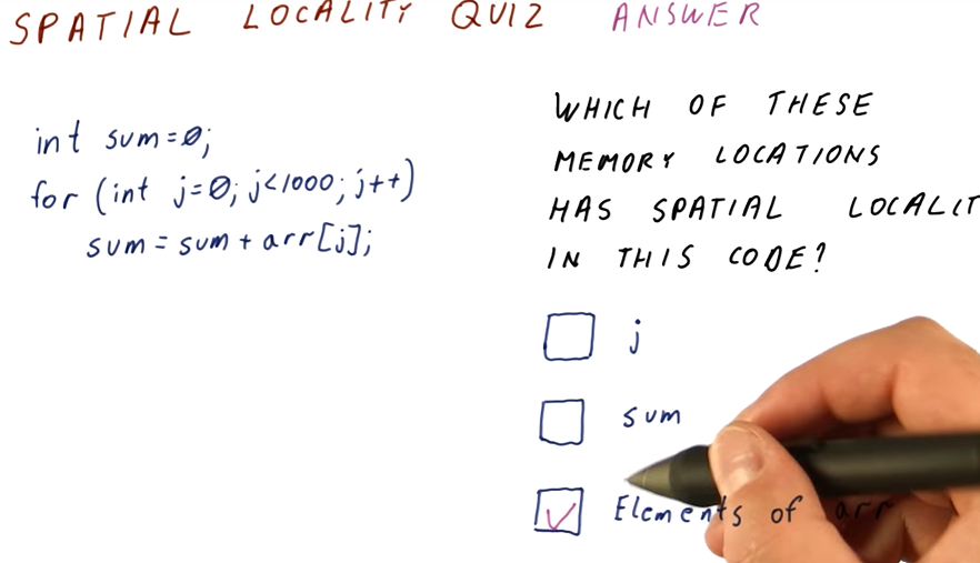
Cache Quiz

The quiz below describes the concept and purpose of a processor cache.

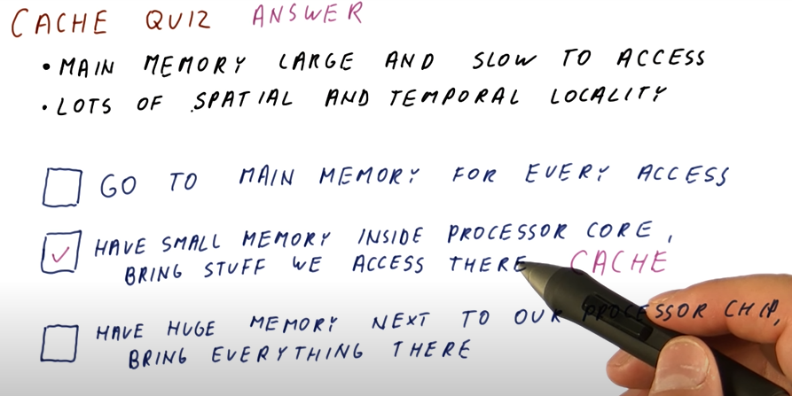
Cache Performance

The below excerpt from the class describes the metrics used to measure cache performance.

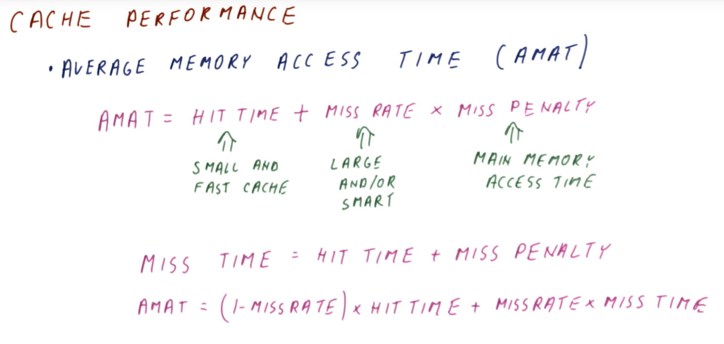
Hit Time Quiz

This quiz asks some common-sense questions about the timing for a well-designed cache.

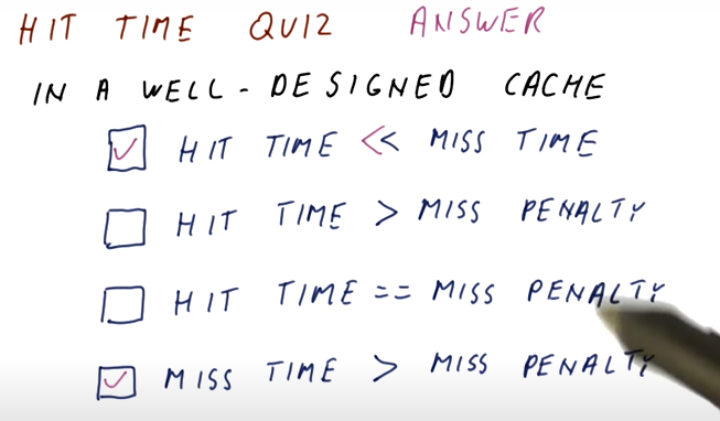
Miss Rate Quiz

This quiz asks common-sense questions on the comparison between hit rate and miss rate.

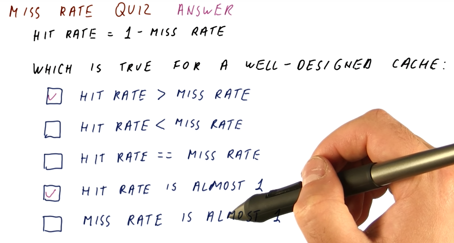
Block Size Quiz

The below quiz covers good use of the cache for variables with specific behaviors.

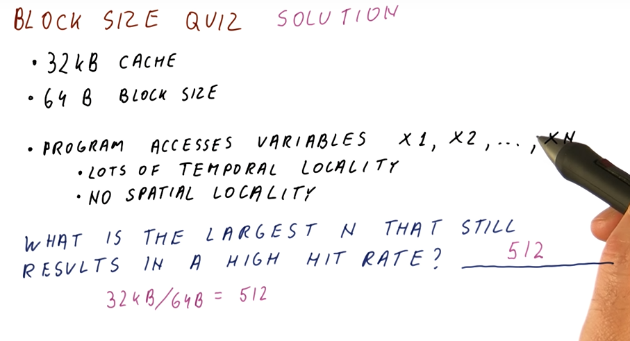
Block Number Quiz

The below quiz shows us how to calculate the block number.

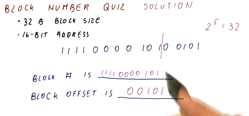
Cache Tags

The below excerpt from the class describes cache tags.

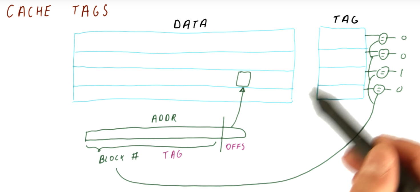
Valid Bit

The below excerpt from the class describes the valid bit.

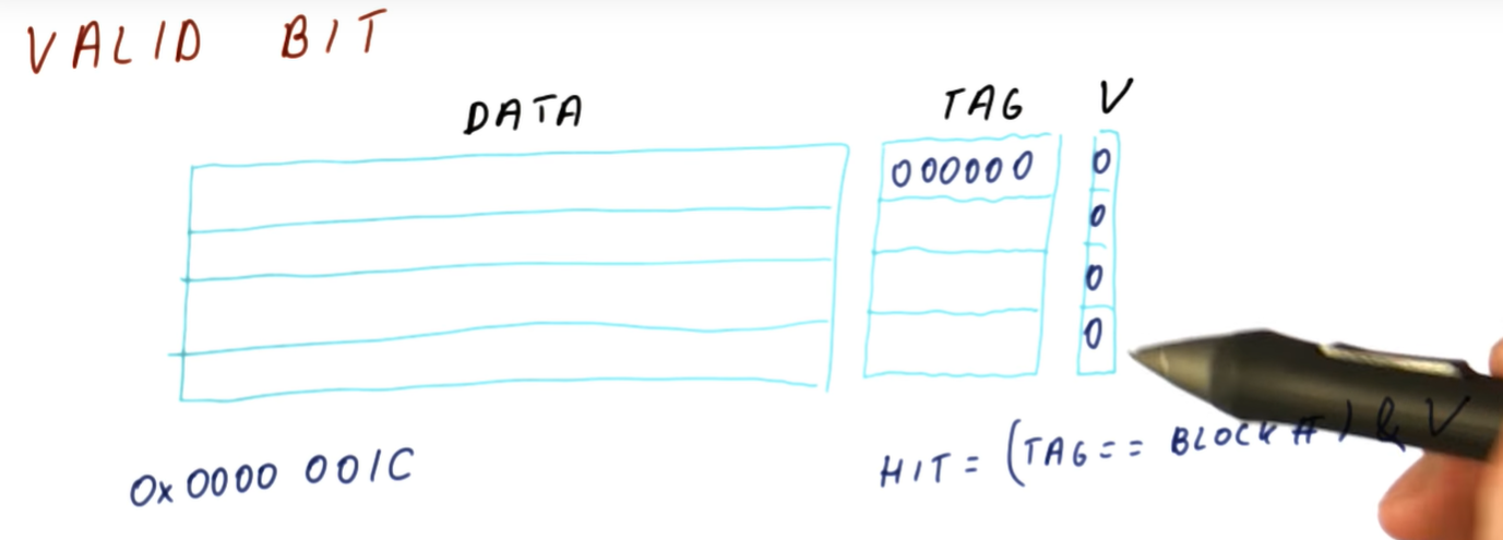
Direct Mapped Cache

The below excerpt from the class describes the direct mapped cache structure.

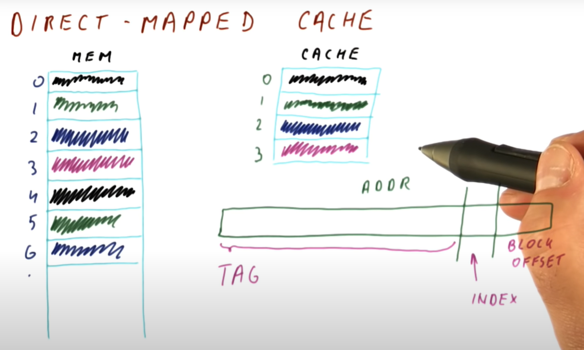
Direct Mapped Cache Quiz

The below quiz demonstrates how to find cache conflicts in direct-mapped caches.

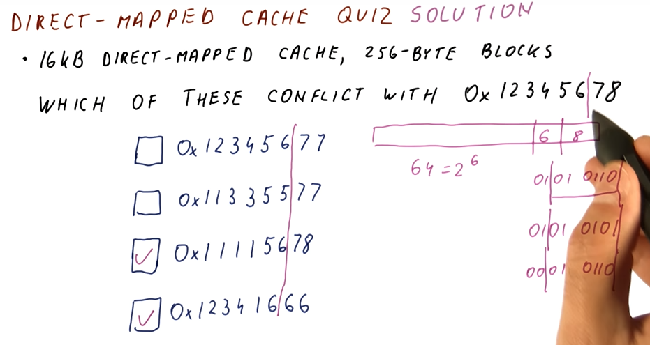
Direct Mapped Cache Quiz

Another direct mapped cache quiz showcasing cache conflicts.

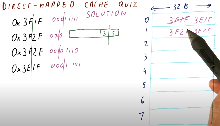
Associative Cache Quiz

The below quiz showcases how we index into an N-way associative cache with an address.

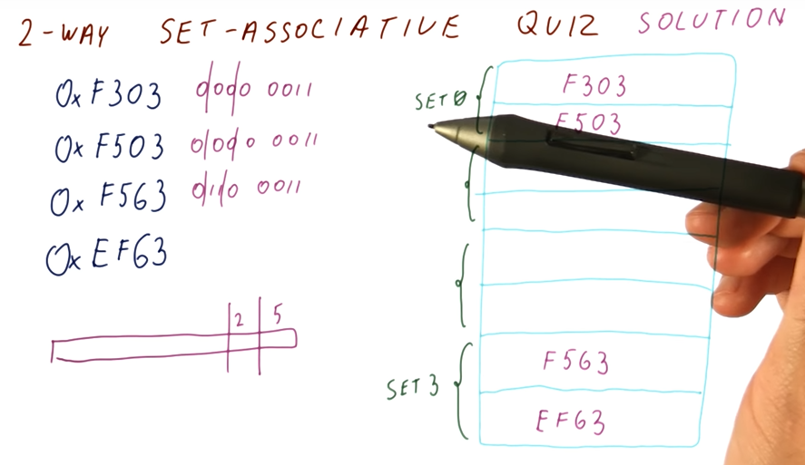
Implementing LRU

The below excerpt from the class describes how the LRU policy is implemented for cache line replacement.

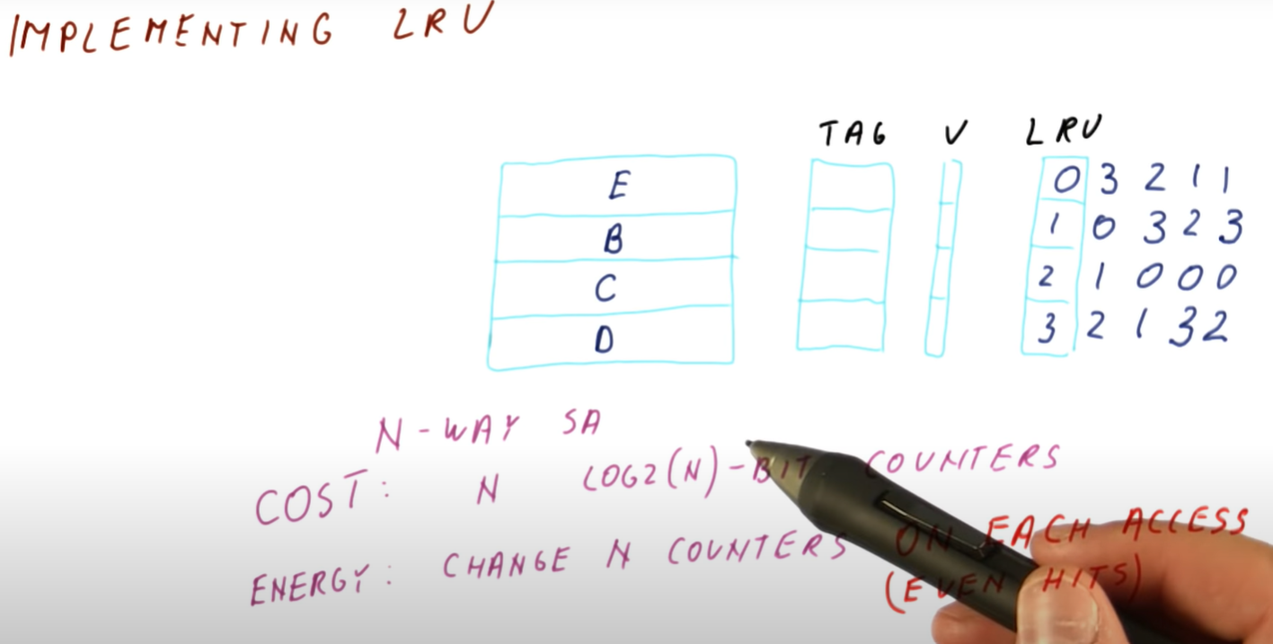
LRU Quiz

The below quiz demonstrates the LRU cache replacement policy.

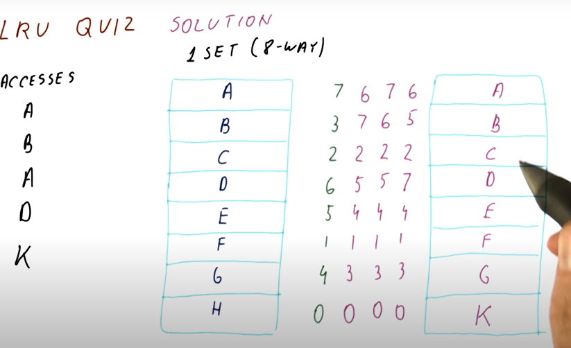
Write Policy

The below excerpt from the lecture provides a good discussion of the differences between cache writing policies.

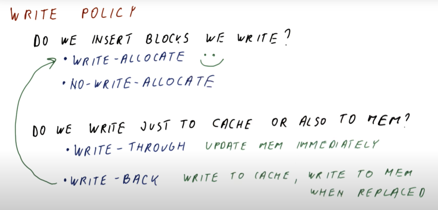
Cache Summary

The below excerpt from the course summarizes the data used to handle an example cache, demonstrating how the cache structure influences the data used to track the tags, indices, etc.

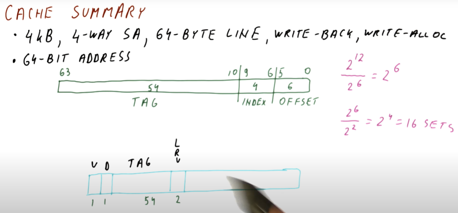
Cache Summary Quiz

Below are the answers to the cache summary quizzes that tie all of these concepts together.

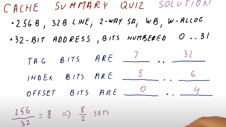
Virtual Memory

This lesson discusses the difference between virtual and physical memory. Virtual memory is used by programs and must be translated to physical memory. Since the translation can be slow, a Translation Look­Aside Buffer (TLB) is used. The notes for this lesson can be found here.

Page Size Quiz

Below is a quiz from the lectures that has us calculate the number of physical memory frames for a system and then the number of page table entries for each process.

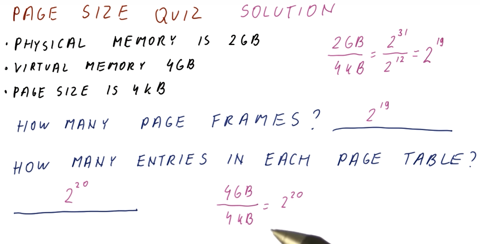
Address Translation Quiz

Below is a quiz from the lectures that demonstrates how to conduct address translation.

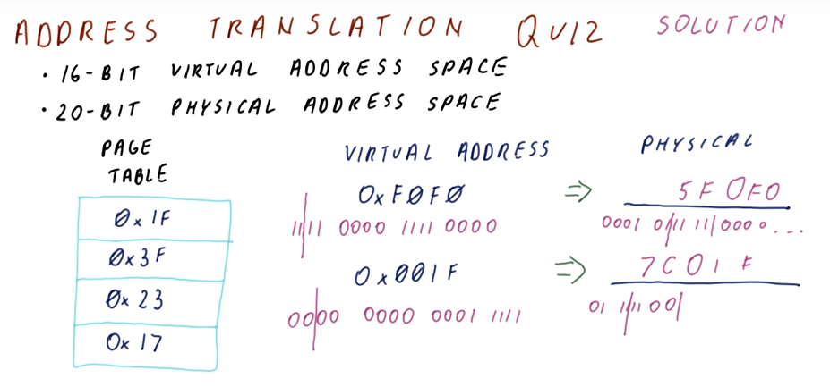
Flat Page Table Size Quiz

Below is a quiz from the lectures that demonstrates how to calculate the size of flat page tables for multiple architectures.

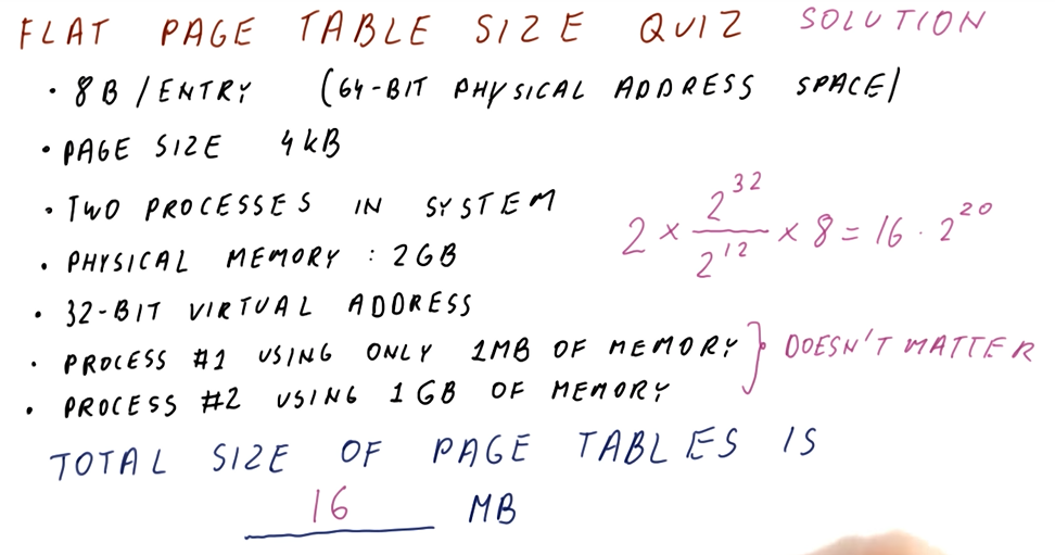
Two Level Page Table Size

The below excerpt from the course describes how we can save memory using multi level page tables.

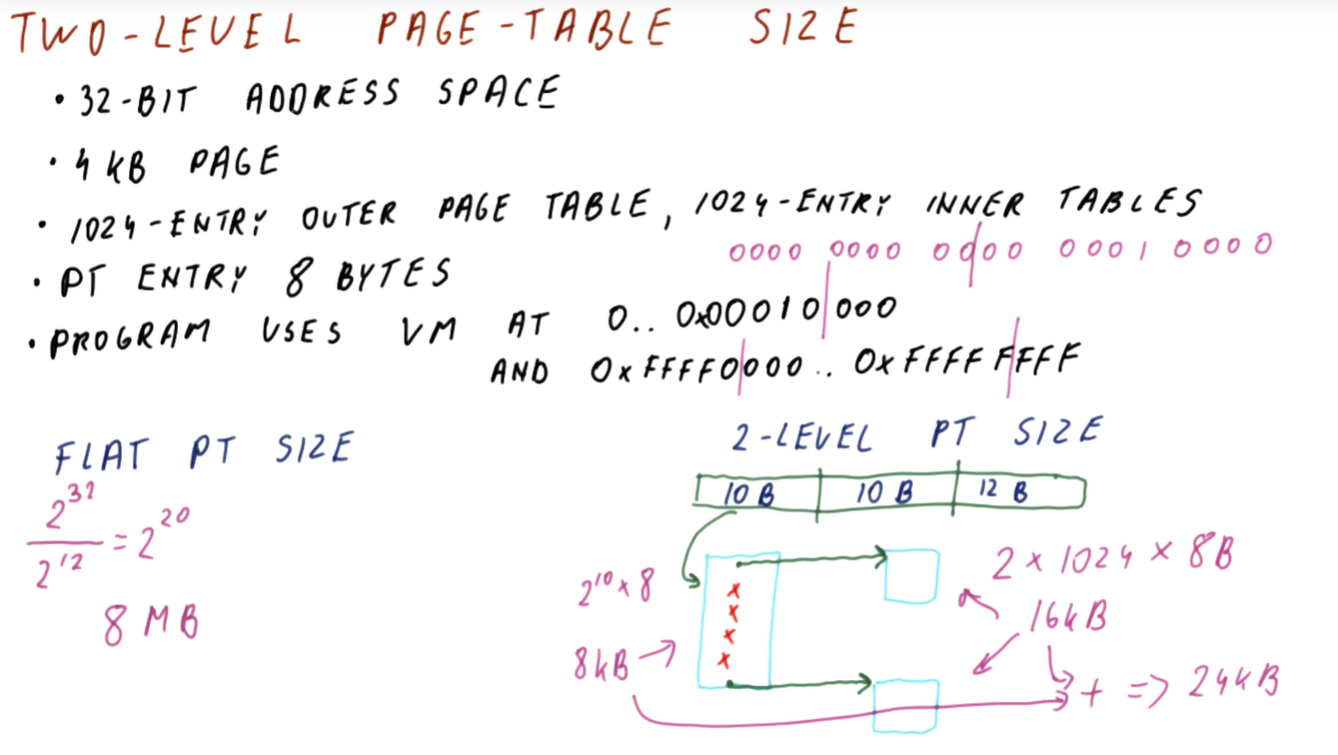
4 Level Page Table Quiz

The below quiz from the lectures demonstrates how to calculate the amount of memory needed for a page table with 4 levels.

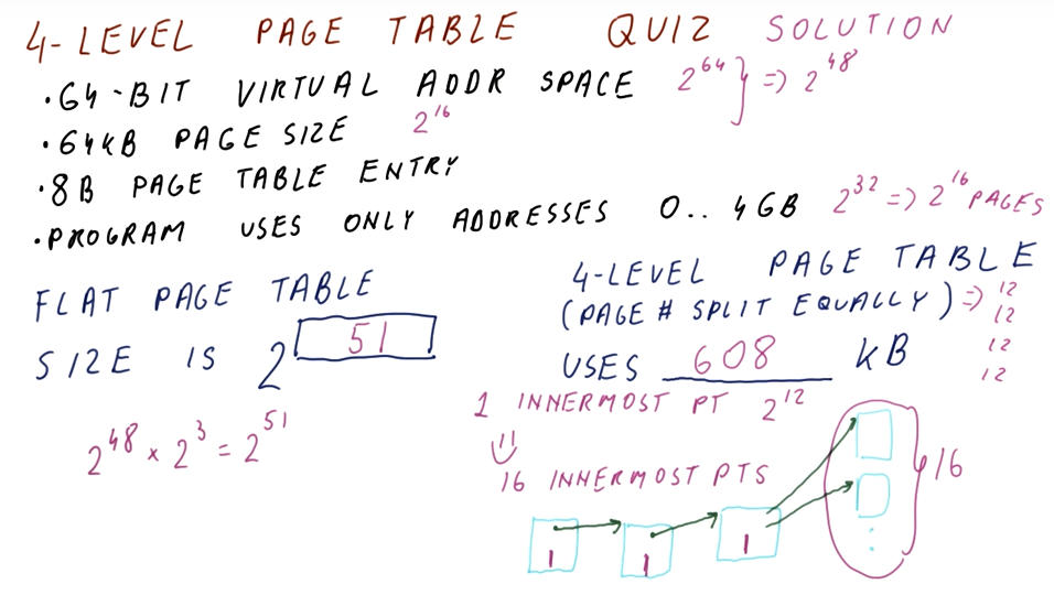
Virtual to Physical Translation Quiz

The below quiz from the lectures demonstrates how to calculate the number of cycles necessary necessary to conduct virtual to physical address translation.

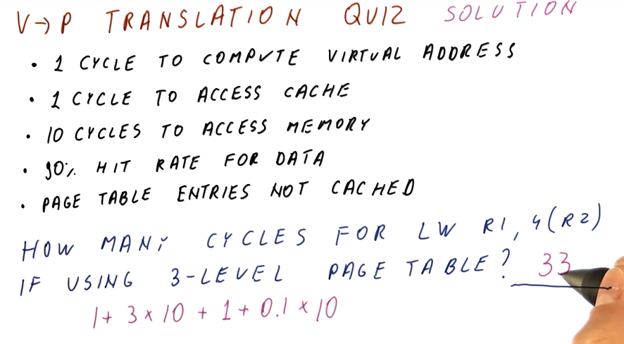
The below quiz from the lectures demonstrates the same as above except the page table entries are cached.

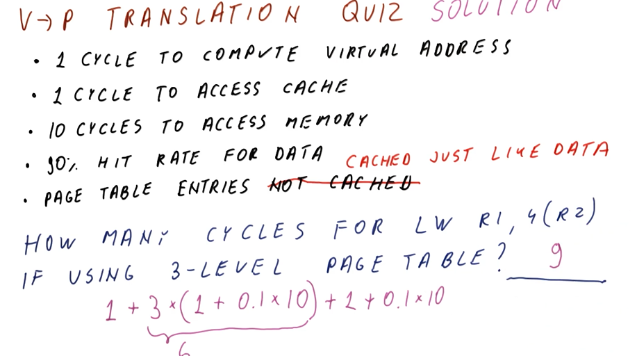
TLB Size Quiz

Below is a quiz from the lectures covering how we can calculate the approx. size of the TLB to achieve similar performance to the cache.

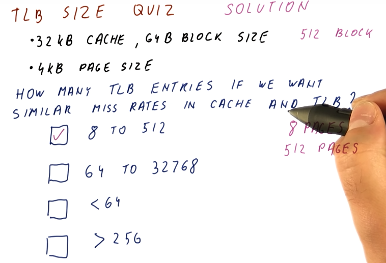
TLB Performance Quiz

Below is quiz demonstrating how to calculate TLB performance for a given set of memory accesses by a program.

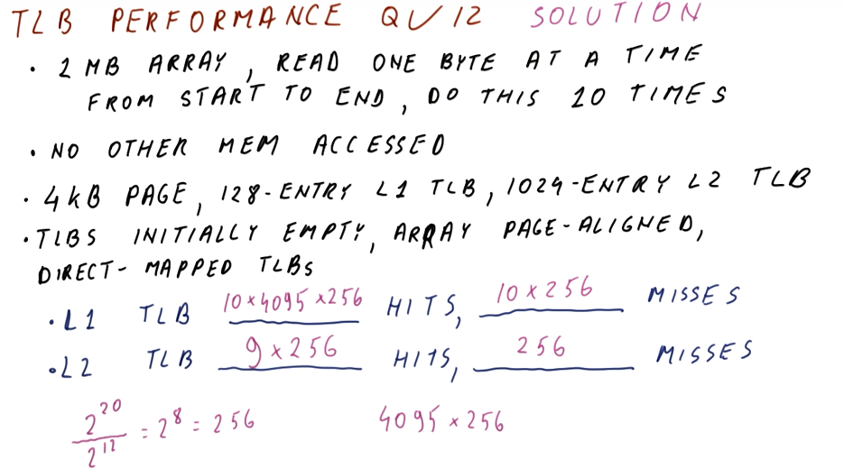
Advanced Caches

Improving the performance of caches is done by improving the hit rate, improving the miss rate, or improving the miss penalty. The methods to implement these improvements in discussed in this lesson. The notes for this lecture can be found here.

VIPT Aliasing Avoidance Quiz

Below is a quiz from the class demonstrating how to calculate the maximum size of a VIPT cache while avoiding aliasing.

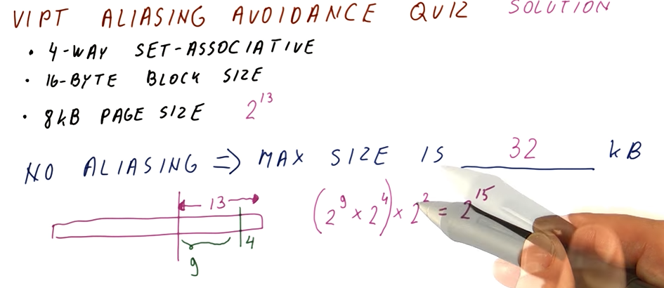
NMRU Quiz

Below is a quiz demonstrating how we can keep track of the hit/misses for an NMRU cache.

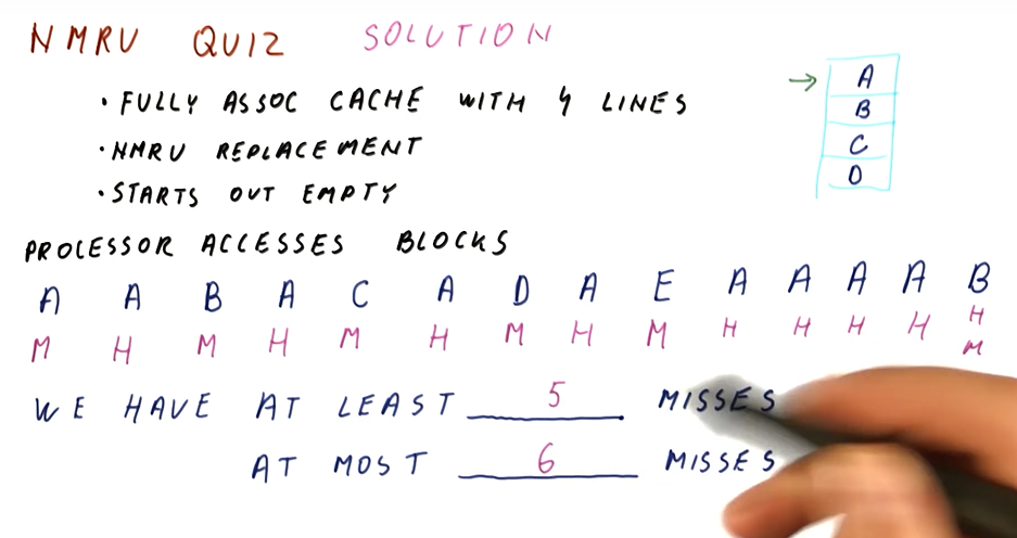
Prefetch Instructions Quiz

Below is a quiz demonstrating how we can calculate how far ahead and whether or not a prefetch should be conducted.

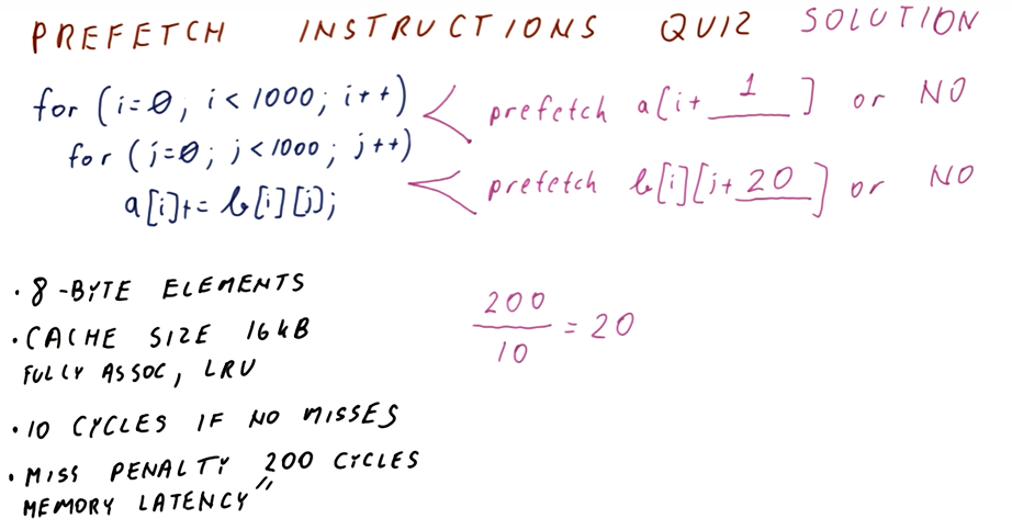
Global and Local Miss Rate Quiz

Below is a quiz demonstrating how to calculate the local and global miss rates for two caches.